TOPPView
Visualizing the data is the first step in quality control, an essential tool in understanding the data, and of course an essential step in pipeline development. OpenMS provides a convenient viewer for some of the data: TOPPView. We will guide you through some of the basic features of TOPPView. Please familiarize yourself with the key controls and visualization methods. We will make use of these later throughout the tutorial. Let’s start with a first look at one of the files of our tutorial data set. Note that conceptually, there are no differences in visualizing metabolomic or proteomic data. Here, we inspect a simple proteomic measurement:
|
|---|
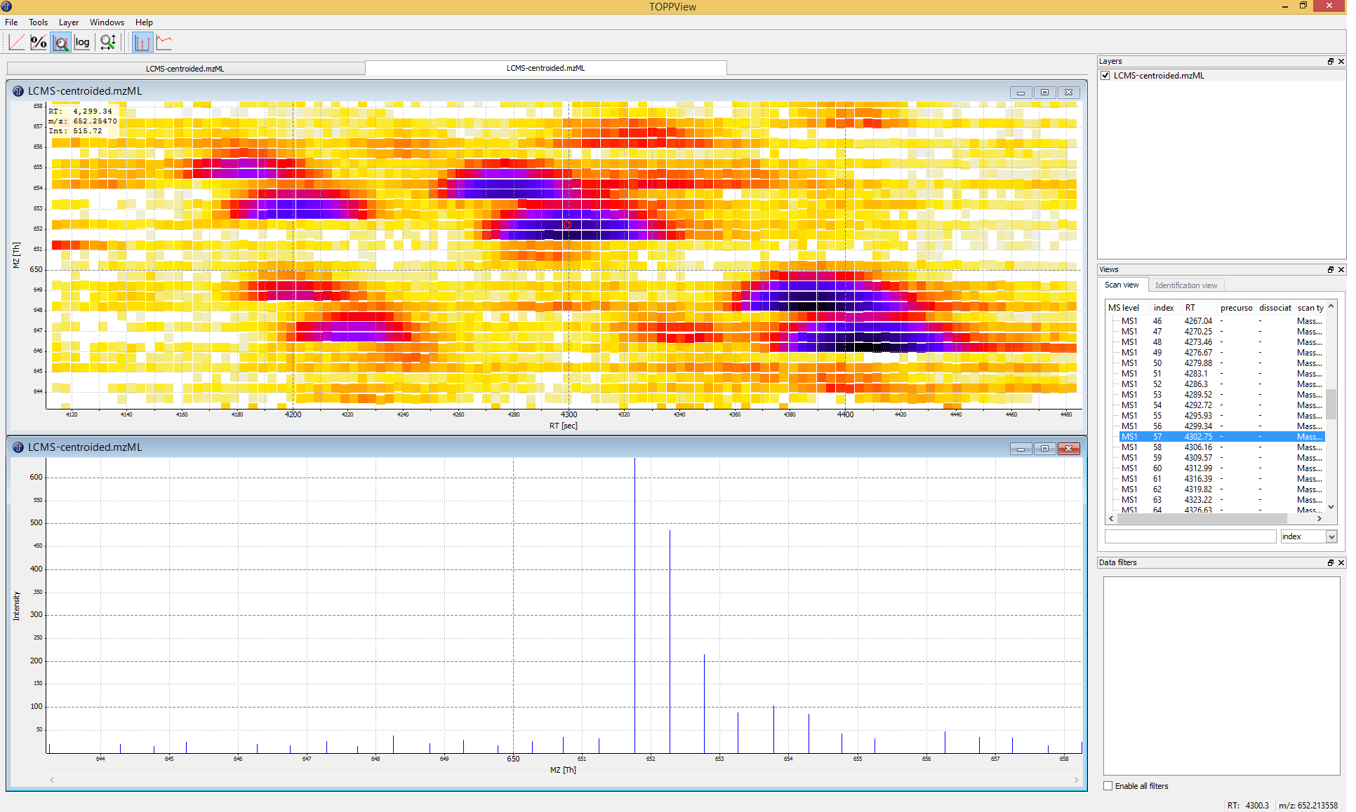
Figure 3: TOPPView, the graphical application for viewing mass spectra and analysis results. Top window shows a small region of a peak map. In this 2D representation of the measured spectra, signals of eluting peptides are colored according to the raw peak intensities. The lower window displays an extracted spectrum (=scan) from the peak map. On the right side, the list of spectra can be browsed. |
|
|---|
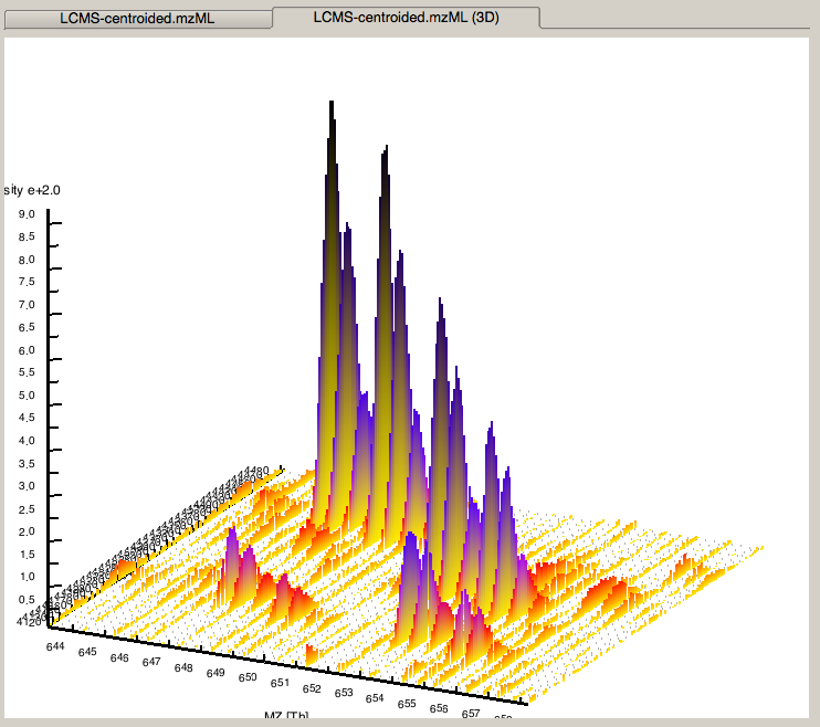
Figure 4: 3D representation of the measured spectra, signals of eluting peptides are colored according to the raw peak intensities. |
Start TOPPView (see Windows’ Start-Menu or
Applications▸OpenMS-3.5.0 on macOS)Go to File > Open File, navigate to the directory where you copied the contents of the USB stick to, and select
Example_Data▸Introduction▸datasets▸small▸velos005614.mzML . This file contains only a reduced LC-MS map of a label-free proteomic platelet measurement recorded on an Orbitrap velos. The other two mzML files contain technical replicates of this experiment. First, we want to obtain a global view on the whole LC-MS map - the default option Map view 2D is the correct one and we can click the Ok button.Play around.
Three basic modes allow you to interact with the displayed data: scrolling, zooming and measuring:
Scroll mode
Is activated by default (though each loaded spectra file is displayed zoomed out first, so you do not need to scroll).
Allows you to browse your data by moving around in RT and m/z range.
When zoomed in, you can scroll through the spectra. Click-drag on the current view.
Arrow keys can be used to scroll the view as well.
Zoom mode
Zooming into the data; either mark an area in the current view with your mouse while holding the left mouse button plus the Ctrl key to zoom to this area or use your mouse wheel to zoom in and out.
All previous zoom levels are stored in a zoom history. The zoom history can be traversed using Ctrl + + or Ctrl + - or the mouse wheel (scroll up and down).
Pressing backspace ← zooms out to show the full LC-MS map (and also resets the zoom history).
Measure mode
It is activated using the ⇧ Shift key.
Press the left mouse button down while a peak is selected and drag the mouse to another peak to measure the distance between peaks.
This mode is implemented in the 1D and 2D mode only.
Right click on your 2D map and select Switch to 3D mode and examine your data in 3D mode (see Fig. 4).
Visualize your data in different intensity normalization modes, use linear, percentage (set intensity axis scale to percentage), snap and log-view (icons on the upper left tool bar). You can hover over the icons for additional information.
Note
On macOS, due to a bug in one of the external libraries used by OpenMS, you will see a small window of the 3D mode when switching to 2D. Close the 3D tab in order to get rid of it.
In TOPPView you can also execute TOPP tools. Go to Tools > Apply tool (whole layer) and choose a TOPP tool (e.g.,
FileInfo) and inspect the results.
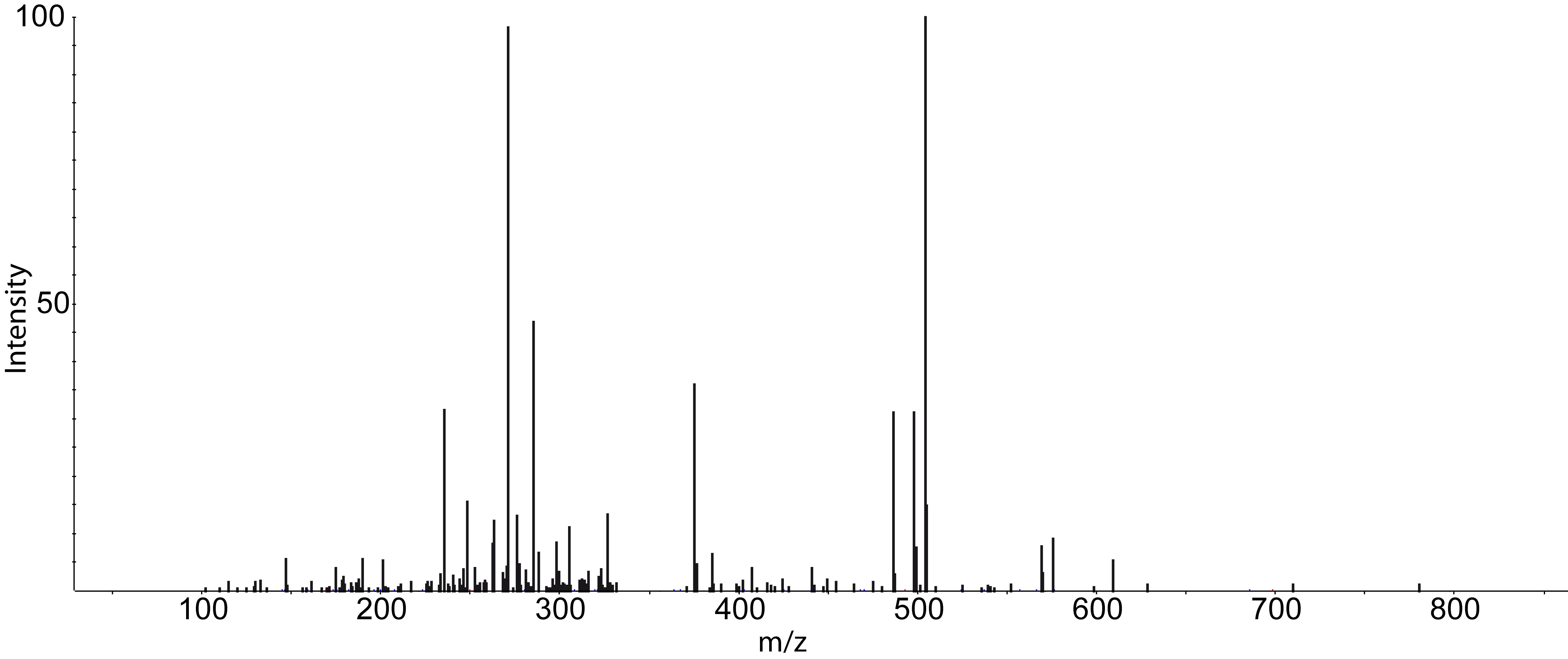
Dependent on your data MS/MS spectra can be visualized as well (see Fig.5) . You can do so, by double-click on the MS/MS spectrum shown in scan view
|
|---|
Figure 5: MS/MS spectrum |