Label-free quantification of peptides and proteins

Introduction

In the following chapter, we will build a workflow with OpenMS / KNIME to quantify a label-free experiment. Label-free quantification is a method aiming to compare the relative amounts of proteins or peptides in two or more samples. We will start from the minimal workflow of the last chapter and, step-by-step, build a label-free quantification workflow.

The complete workflow can be downloaded here as well.

Peptide identification

As a start, we will extend the minimal workflow so that it performs a peptide identification using the Comet search engine. Comet is included in the OpenMS installation, so you do not need to download and install it yourself.

Let’s start by replacing the input files in our Input Files node by the three mzML files in Example Data > Labelfree > datasets > lfqxspikeinxdilutionx1-3.mzML. This is a reduced toy dataset where each of the three runs contains a constant background of S. pyogenes peptides as well as human spike-in peptides in different concentrations. [1]

• Instead of FileFilter, we want to perform Comet identification, so we simply replace the FileFilter node with the CometAdapter node Community Nodes > OpenMSThirdParty > Identification, and we are almost done. Just make sure you have connected the ZipLoopStart node with the in (top) port of the CometAdapter node.

• Comet, like most mass spectrometry identification engines, relies on searching the input spectra against sequence databases. Thus, we need to introduce a search database input. As we want to use the same search database for all of our input files, we can just add a single File Importer node to the workflow and connect it directly with the CometAdapter database (middle) port. KNIME will automatically reuse this Input node each time a new ZipLoop iteration is started. In order to specify the database, select Example_Data▸Labelfree▸databases▸
  ▸s_pyo_sf370_potato_human_target_decoy_with_contaminants.fasta

• Connect the out port of the CometAdapter to ZipLoopEnd and we have a very basic peptide identification workflow.

  Note

  You might also want to save your new identification workflow under a different name. Have a look at duplicating workflows for information on how to create copies of workflows.

• The result of a single Comet run is basically a number of peptide-spectrum-matches (PSM) with a score each, and these will be stored in an idXML file. Now we can run the pipeline and after execution is finished, we can have a first look at the the results: just open the output folder with a file browser and from there open one of the three input mzML’s in TOPPView.

• Here, annotate this spectrum data file with the peptide identification results. Choose Tools > Annonate with identification from the menu and select the idXML file that CometAdapter generated (it is located within the output directory that you specified when starting the pipeline).

• On the right, select the tab Identification view. All identified peptides can be seen using this view. User can also browse the corresponding MS2 spectra.

  Note

  Opening the output file of CometAdapter (the idXML file) directly is also possible, but unless you REALLY like XML, reading idXML files is less useful.

• The search results stored in the idXML file can also be read back into a KNIME table for inspection and subsequent analyses: Add a TextExporter node from Community Nodes > OpenMS > File Handling to your workflow and connect the output port of your CometAdapter (the same port ZipLoopEnd is connected to) to its input port. This tool will convert the idXML file to a more human-readable text file which can also be read into a KNIME table using the IDTextReader node. Add an IDTextReader node(Community Nodes > OpenMS > Conversion) after TextExporter and execute it. Now you can right click IDTextReader and select ID Table to browse your peptide identifications.

• From here, you can use all the tools KNIME offers for analyzing the data in this table. As a simple example, add a Histogram node (from category Views) node after IDTextReader, double-click it, select peptide_charge as Dimension, click Save and Execute to generate a plot showing the charge state distribution of your identifications.

In the next step, we will tweak the parameters of Comet to better reflect the instrument’s accuracy. Also, we will extend our pipeline with a false discovery rate (FDR) filter to retain only those identifications that will yield an FDR of < 1 %.

• Open the configuration dialog of CometAdapter. The dataset was recorded using an LTQ Orbitrap XL mass spectrometer, set the precursor_mass_tolerance to 5 and precursor_error_units to ppm.

  Note

  Whenever you change the configuration of a node, the node as well as all its successors will be reset to the Configured state (all node results are discarded and need to be recalculated by executing the nodes again).

• Make sure that Carbamidomethyl (C) is set as fixed modification and Oxidation(M) as variable modification.

  Note

  To add a modification click on the empty value field in the configuration dialog to open the list editor dialog. In the new dialog click Add. Then select the newly added modification to open the drop down list where you can select the the correct modification.

• A common step in analysis is to search not only against a regular protein database, but to also search against a decoy database for FDR estimation. The fasta file we used before already contains such a decoy database. For OpenMS to know which Comet PSM came from which part of the file (i.e. target versus decoy), we have to index the results. To this end, extend the workflow with a PeptideIndexer node Community Nodes > OpenMS > ID Processing. This node needs the idXML as input as well as the database file (see below figure).

  Tip

  You can direct the files of an File Importer node to more than just one destination port.

• The decoys in the database are prefixed with “DECOY_”, so we have to set decoy_string to DECOY_ and decoy_string_position to prefix in the configuration dialog of PeptideIndexer.

• Now we can go for the FDR estimation, which the FalseDiscoveryRate node will calculate for us (you will find it in Community Nodes > OpenMS > Identification Processing). FalseDiscoveryRate is meant to be run on data with protein inferencences (more on that later), in order to just use it for peptides, open the configure window, select “show advanced parameter” and toggle “force” to true.

• In order to set the FDR level to 1%, we need an IDFilter node from Community Nodes > OpenMS > Identification Processing. Configuring its parameter score→pep to 0.01 will do the trick. The FDR calculations (embedded in the idXML) from the FalseDiscoveryRate node will go into the in port of the IDFilter node.

• Execute your workflow and inspect the results using IDTextReader like you did before. How many peptides did you identify at this FDR threshold?

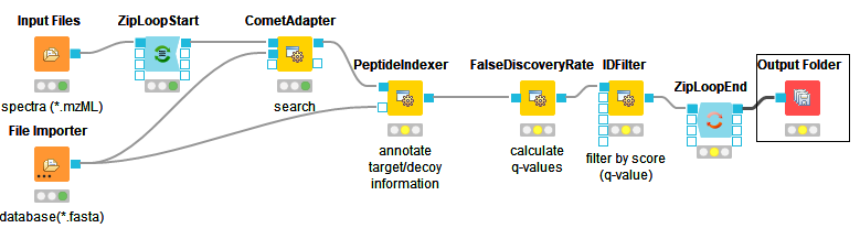
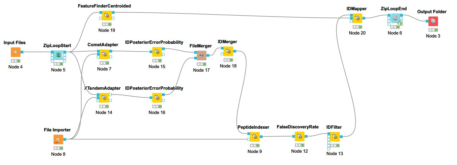
The below images shows Comet ID pipeline including FDR filtering.

Figure 12: Comet ID pipeline including FDR filtering

Bonus task: Identification using several search engines

Note

If you are ahead of the tutorial or later on, you can further improve your FDR identification workflow by a so-called consensus identification using several search engines. Otherwise, just continue with quantification.

It has become widely accepted that the parallel usage of different search engines can increase peptide identification rates in shotgun proteomics experiments. The ConsensusID algorithm is based on the calculation of posterior error probabilities (PEP) and a combination of the normalized scores by considering missing peptide sequences.

• Next to the CometAdapter add a XTandemAdapter Community Nodes > OpenMSThirdParty > Identification of Proteins > Peptides(SearchEngines) node and set its parameters and ports analogously to the CometAdapter. In XTandem, to get more evenly distributed scores, we decrease the number of candidates a bit by setting the precursor mass tolerance to 5 ppm and the fragment mass tolerance to 0.1 Da.

• To calculate the PEP, introduce a IDPosteriorErrorProbability Community Nodes > OpenMS > Identification Processing node to the output of each ID engine adapter node. This will calculate the PEP to each hit and output an updated idXML.

• To create a consensus, we must first merge these two files with a FileMerger node Community Nodes > GenericKnimeNode > Flow so we can then merge the corresponding IDs with a IDMerger Community Nodes > OpenMS > File Handling.

• Now we can create a consensus identification with the ConsensusID Community Nodes > OpenMS > Identification Processing node. We can connect this to the PeptideIndexer and go along with our existing FDR filtering.

  Note

  By default, X!Tandem takes additional enzyme cutting rules into consideration (besides the specified tryptic digest). Thus for the tutorial files, you have to set PeptideIndexer’s enzyme→specificity parameter to none to accept X!Tandem’s non-tryptic identifications as well.

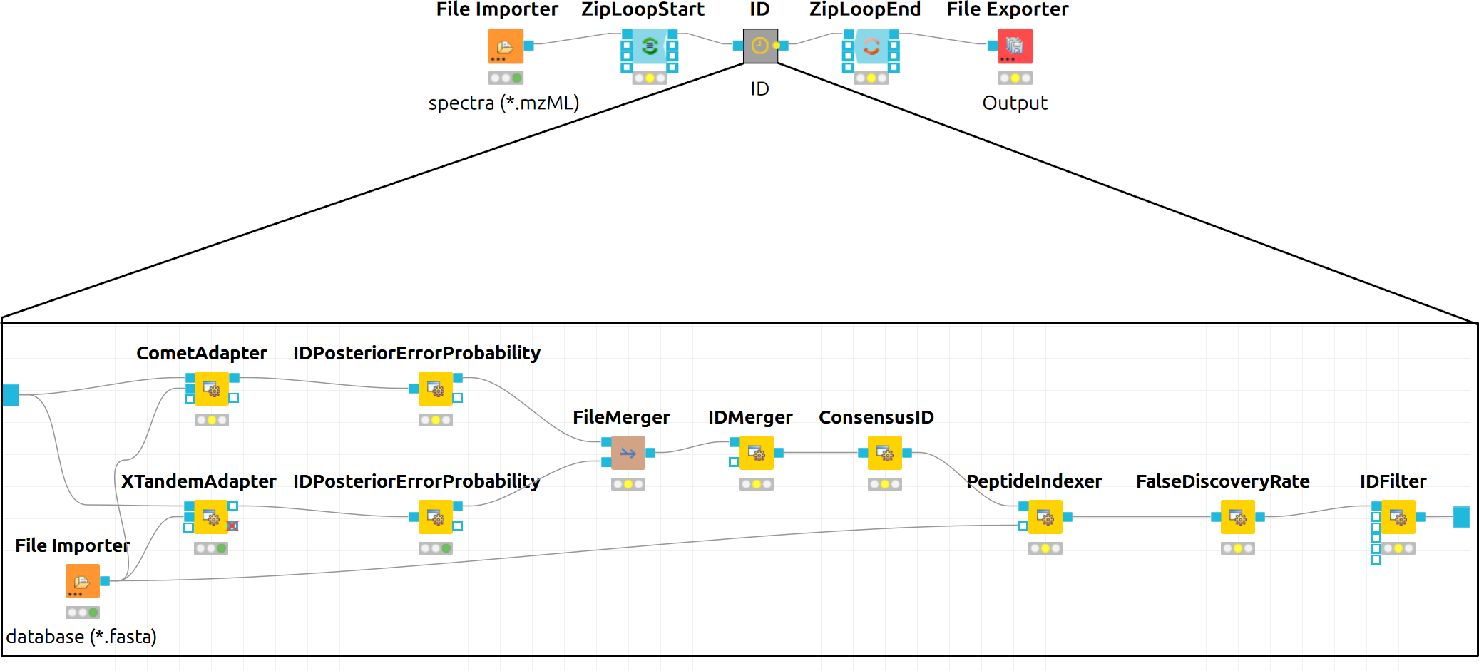
In the end, the ID processing part of the workflow can be collapsed into a Metanode to keep the structure clean (see below figure which shows complete consensus identification workflow).

Figure 13: Complete consensus identification workflow

Feature Mapping

Now that we have successfully constructed a peptide identification pipeline, we can assign this information to the corresponding feature signals.

• Add a FeatureFinderCentroided node from Community Nodes > OpenMS > Quantitation which gets input from the first output port of the ZipLoopStart node. Also, add an IDMapper node (from Community Nodes > OpenMS > Identification Processing ) which receives input from the FeatureFinderCentroided node (Port 1) and the IDFilter node (Port 0). The output of the IDMapper node is then connected to an in port of the ZipLoopEnd node.

• FeatureFinderCentroided finds and quantifies peptide ion signals contained in the MS1 data. It reduces the entire signal, i.e., all peaks explained by one and the same peptide ion signal, to a single peak at the maximum of the chromatographic elution profile of the monoisotopic mass trace of this peptide ion and assigns an overall intensity.

• FeatureFinderCentroided produces a featureXML file as output, containing only quantitative information of so-far unidentified peptide signals. In order to annotate these with the corresponding ID information, we need the IDMapper node.

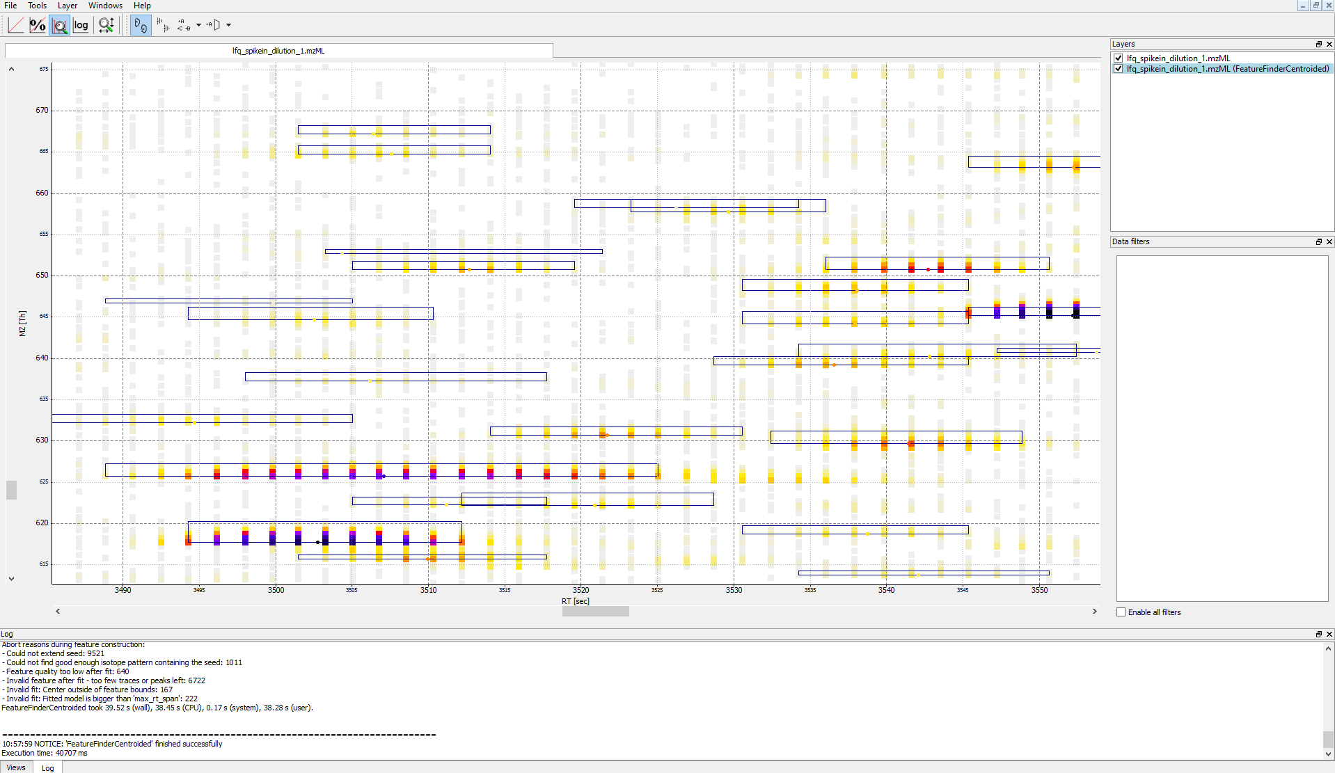
• Run your pipeline and inspect the results of the IDMapper node in TOPPView. Open the mzML file of your data to display the raw peak intensities.

• To assess how well the feature finding worked, you can project the features contained in the featureXML file on the raw data contained in the mzML file. To this end, open the featureXML file in TOPPView by clicking on File Open file and add it to a new layer ( Open in New layer ). The features are now visualized on top of your raw data. If you zoom in on a small region, you should be able to see the individual boxes around features that have been detected (see Fig. 14). If you hover over the the feature centroid (small circle indicating the chromatographic apex of monoisotopic trace) additional information of the feature is displayed.

  || |:–:| |Figure 14: Visualization of detected features (boxes) in TOPPView|

  Note

  The chromatographic RT range of a feature is about 30-60 s and its m/z range around 2.5 m/z in this dataset. If you have trouble zooming in on a feature, select the full RT range and zoom only into the m/z dimension by holding down Ctrl ( cmd ⌘ on macOS) and repeatedly dragging a narrow box from the very left to the very right

• You can see which features were annotated with a peptide identification by first selecting the featureXML file in the Layers window on the upper right side and then clicking on the icon with the letters A, B and C on the upper icon bar. Now, click on the small triangle next to that icon and select Peptide identification.

The following image shows the final constructed workflow:

Figure 15: Extended workflow featuring peptide identification and feature mapping.

Combining features across several label-free experiments

So far, we successfully performed peptide identification as well as feature mapping on individual LC-MS runs. For differential label-free analyses, however, we need to identify and map corresponding signals in different experiments and link them together to compare their intensities. Thus, we will now run our pipeline on all three available input files and extend it a bit further, so that it is able to find and link features across several runs.

Figure 16: Complete identification and label-free feature mapping workflow. The identification nodes are grouped together as ID metanode.

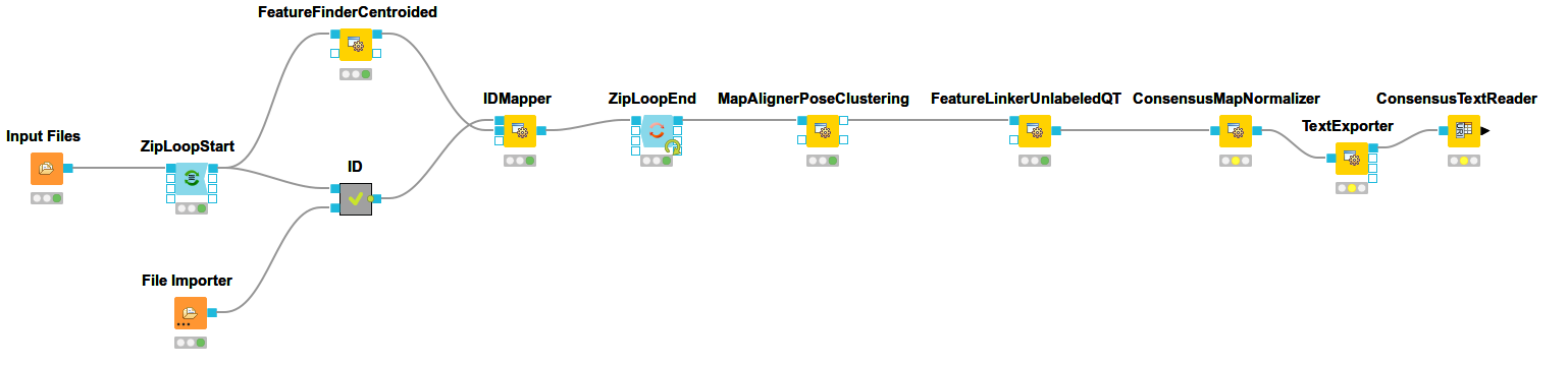
• To link features across several maps, we first have to align them to correct for retention time shifts between the different label-free measurements. With the MapAlignerPoseClustering node in Community Nodes > OpenMS > Map Alignment, we can align corresponding peptide signals to each other as closely as possible by applying a transformation in the RT dimension.

  Note

  MapAlignerPoseClustering consumes several featureXML files and its output should still be several featureXML files containing the same features, but with the transformed RT values. In its configuration dialog, make sure that OutputTypes is set to featureXML.

• With the FeatureLinkerUnlabeledQT node in Community Nodes > OpenMS > Map Alignment, we can then perform the actual linking of corresponding features. Its output is a consensusXML file containing linked groups of corresponding features across the different experiments.

• Since the overall intensities can vary a lot between different measurements (for example, because the amount of injected analytes was different), we apply the ConsensusMapNormalizer node in Community Node > OpenMS > Map Alignment as a last processing step. Configure its parameters with setting algorithm_type to median. It will then normalize the maps in such a way that the median intensity of all input maps is equal.

• Export the resulting normalized consensusXML file to a csv format using the TextExporter node.

• Use the ConsensusTextReader node in Community Nodes > OpenMS > Conversion to convert the output into a KNIME table. After running the node you can view the KNIME table by right-clicking on the ConsensusTextReader node and selecting Consensus Table. Every row in this table corresponds to a so-called consensus feature, i.e., a peptide signal quantified across several runs. The first couple of columns describe the consensus feature as a whole (average RT and m/z across the maps, charge, etc.). The remaining columns describe the exact positions and intensities of the quantified features separately for all input samples (e.g., intensity_0 is the intensity of the feature in the first input file). The last 11 columns contain information on peptide identification.

  Note

  You can specify the desired column separation character in the parameter settings (by default, it is set to “ ” (a space)). The output file of TextExporter can also be opened with external tools, e.g., Microsoft Excel, for downstream statistical analyses.

Basic data analysis in KNIME

In this section we are going to use the output of the ConsensusTextReader for downstream analysis of the quantification results:

• Let’s say we want to plot the log intensity distributions of the human spike-in peptides for all input files. In addition, we will plot the intensity distributions of the background peptides.

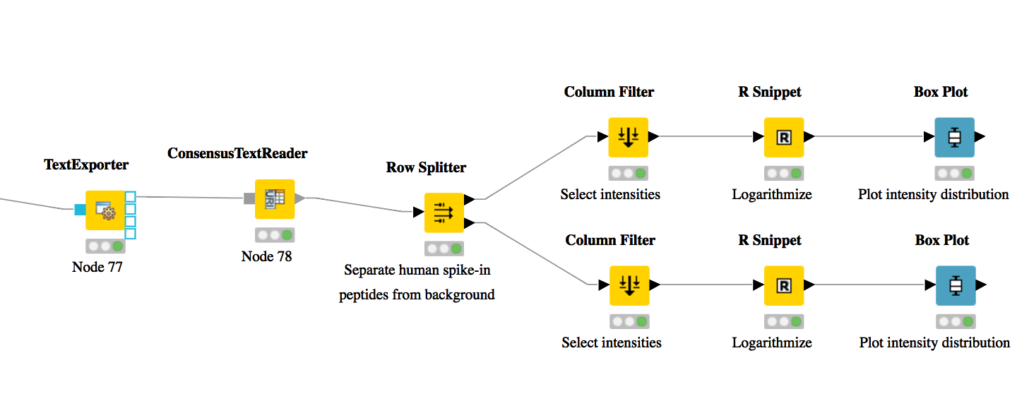
• As shown in Fig. 17, add a Row Splitter node (Data Manipulation > Row > Filter) after the ConsensusTextReader node. Double-click it to configure. The human spike-in peptides have accessions starting with “hum”. Thus, set the column to apply the test to accessions, select pattern matching as matching criterion, enter hum* into the corresponding text field, and check the contains wild cards box. Press OK and execute the node.

• Row Splitter produces two output tables: the first one contains all rows from the input table matching the filter criterion, and the second table contains all other rows. You can inspect the tables by right-clicking and selecting Filtered and Filtered Out. The former table should now only contain peptides with a human accession, whereas the latter should contain all remaining peptides (including unidentified ones).

• Now, since we only want to plot intensities, we can add a Column Filter node by going to Data Manipulation > Column Filter. Connect its input port to the Filtered output port of the Row Filter node, and open its configuration dialog. We could either manually select the columns we want to keep, or, more elegantly, select Wildcard/Regex Selection and enter intensity_? as the pattern. KNIME will interactively show you which columns your pattern applies to while you’re typing.

• Since we want to plot log intensities, we will now compute the log of all intensity values in our table. The easiest way to do this in KNIME is a small piece of R code. Add an R Snippet node R after Column Filter and double-click to configure. In the R Script text editor, enter the following code:

  x <- knime.in       # store copy of input table in x
  
  x[x == 0] <- NA     # replace all zeros by NA (= missing value)
  
  x <- log10(x)       # compute log of all values
  knime.out <- x      # write result to output table
  

• Now we are ready to plot! Add a Box Plot (JavaScript) node Views -JavaScript after the R Snippet node, execute it, and open its view. If everything went well, you should see a significant fold change of your human peptide intensities across the three runs.

• To verify that the concentration of background peptides is constant in all three runs, copy and paste the three nodes after Row Splitter and connect the duplicated Column Filter to the second output port (Filtered Out) of Row Splitter, as shown in Fig. 17. Execute and open the view of your second Box Plot.

You have now constructed an entire identification and label-free feature mapping workflow including a simple data analysis using KNIME. The final workflow should like the workflow shown in the following image:

Figure 17: Simple KNIME data analysis example for LFQ

Extending the LFQ workflow by protein inference and quantification

We have made the following changes compared to the original label-free quantification workflow from the last chapter:

• First, we have added a ProteinQuantifier node and connected its input port to the output port of the ConsensusMapNormalizer node.

• This already enables protein quantification. ProteinQuantifier quantifies peptides by summarizing over all observed charge states and proteins by summarizing over their quantified peptides. It stores two output files, one for the quantified peptides and one for the proteins.

• In this example, we consider only the protein quantification output file, which is written to the first output port of ProteinQuantifier.

• Because there is no dedicated node in KNIME to read back the ProteinQuantifier output file format into a KNIME table, we have to use a workaround. Here, we have added an additional URI Port to Variable node which converts the name of the output file to a so-called “flow variable” in KNIME. This variable is passed on to the next node CSV Reader, where it is used to specify the name of the input file to be read. If you double-click on CSV Reader, you will see that the text field, where you usually enter the location of the CSV file to be read, is greyed out. Instead, the flow variable is used to specify the location, as indicated by the small green button with the “v=?” label on the right.

• The table containing the ProteinQuantifier results is filtered one more time in order to remove decoy proteins. You can have a look at the final list of quantified protein groups by right-clicking the Row Filter and selecting Filtered.

• By default, i.e., when the second input port protein_groups is not used, ProteinQuantifier quantifies proteins using only the unique peptides, which usually results in rather low numbers of quantified proteins.

• In this example, however, we have performed protein inference using Fido and used the resulting protein grouping information to also quantify indistinguishable proteins. In fact, we also used a greedy method in FidoAdapter (parameter greedy_group_resolution) to uniquely assign the peptides of a group to the most probable protein(s) in the respective group. This boosts the number of quantifications but slightly raises the chances to yield distorted protein quantities.

• As a prerequisite for using FidoAdapter, we have added an IDPosteriorErrorProbability node within the ID meta node, between the XTandemAdapter (note the replacement of OMSSA because of ill-calibrated scores) and PeptideIndexer. We have set its parameter prob_correct to true, so it computes posterior probabilities instead of posterior error probabilities (1 - PEP). These are stored in the resulting idXML file and later on used by the Fido algorithm. Also note that we excluded FDR filtering from the standard meta node. Harsh filtering before inference impacts the calibration of the results. Since we filter peptides before quantification though, no potentially random peptides will be included in the results anyway.

• Next, we have added a third outgoing connection to our ID meta node and connected it to the second input port of ZipLoopEnd. Thus, KNIME will wait until all input files have been processed by the loop and then pass on the resulting list of idXML files to the subsequent IDMerger node, which merges all identifications from all idXML files into a single idXML file. This is done to get a unique assignment of peptides to proteins over all samples.

• Instead of the meta node Protein inference with FidoAdapter, we could have just used a FidoAdapter node ( Community Nodes > OpenMS > Identification Processing). However, the meta node contains an additional subworkflow which, besides calling FidoAdapter, performs a statistical validation (e.g. (pseudo) receiver operating curves; ROCs) of the protein inference results using some of the more advanced KNIME and R nodes. The meta node also shows how to use MzTabExporter and MzTabReader.

Statistical validation of protein inference results

In the following section, we will explain the subworkflow contained in the Protein inference with FidoAdapter meta node.

Data preparation

For downstream analysis on the protein ID level in KNIME, it is again necessary to convert the idXML-file-format result generated from FidoAdapter into a KNIME table.

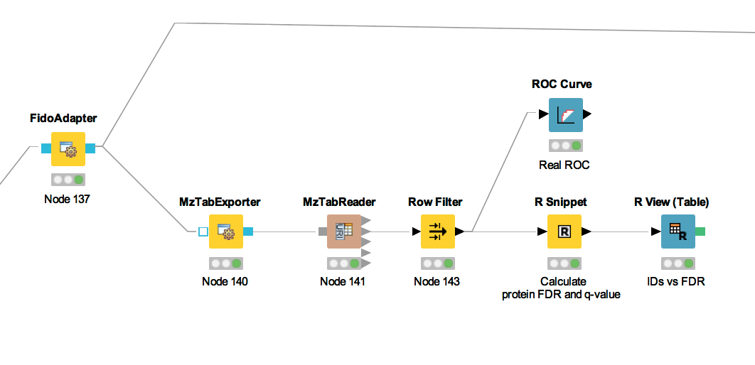
• We use the MzTabExporter to convert the inference results from FidoAdapter to a human readable, tab-separated mzTab file. mzTab contains multiple sections, that are all exported by default, if applicable. This file, with its different sections can again be read by the MzTabReader that produces one output in KNIME table format (triangle ports) for each section. Some ports might be empty if a section did not exist. Of course, we continue by connecting the downstream nodes with the protein section output (second port).

• Since the protein section contains single proteins as well as protein groups, we filter them for single proteins with the standard Row Filter.

ROC curve of protein ID

ROC Curves (Receiver Operating Characteristic curves) are graphical plots that visualize sensitivity (true-positive rate) against fall-out (false positive rate). They are often used to judge the quality of a discrimination method like e.g., peptide or protein identification engines. ROC Curve already provides the functionality of drawing ROC curves for binary classification problems. When configuring this node, select the opt_global_target_decoy column as the class (i.e. target outcome) column. We want to find out, how good our inferred protein probability discriminates between them, therefore add best_search_engine_score[1] (the inference engine score is treated like a peptide search engine score) to the list of ”Columns containing positive class probabilities”. View the plot by right-clicking and selecting View: ROC Curves. A perfect classifier has an area under the curve (AUC) of 1.0 and its curve touches the upper left of the plot. However, in protein or peptide identification, the ground-truth (i.e., which target identifications are true, which are false) is usually not known. Instead, so called pseudoROC Curves are regularly used to plot the number of target proteins against the false discovery rate (FDR) or its protein-centric counterpart, the q-value. The FDR is approximated by using the target-decoy estimate in order to distinguish true IDs from false IDs by separating target IDs from decoy IDs.

Posterior probability and FDR of protein IDs

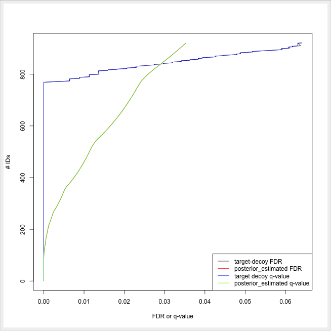
ROC curves illustrate the discriminative capability of the scores of IDs. In the case of protein identifications, Fido produces the posterior probability of each protein as the output score. However, a perfect score should not only be highly discriminative (distinguishing true from false IDs), it should also be “calibrated” (for probability indicating that all IDs with reported posterior probability scores of 95% should roughly have a 5% probability of being false. This implies that the estimated number of false positives can be computed as the sum of posterior error probabilities ( = 1 - posterior probability) in a set, divided by the number of proteins in the set. Thereby a posterior-probability-estimated FDR is computed which can be compared to the actual target-decoy FDR. We can plot calibration curves to help us visualize the quality of the score (when the score is interpreted as a probability as Fido does), by comparing how similar the target-decoy estimated FDR and the posterior probability estimated FDR are. Good results should show a close correspondence between these two measurements, although a non-correspondence does not necessarily indicate wrong results.

The calculation is done by using a simple R script in R snippet. First, the target decoy protein FDR is computed as the proportion of decoy proteins among all significant protein IDs. Then posterior probabilistic-driven FDR is estimated by the average of the posterior error probability of all significant protein IDs. Since FDR is the property for a group of protein IDs, we can also calculate a local property for each protein: the q-value of a certain protein ID is the minimum FDR of any groups of protein IDs that contain this protein ID. We plot the protein ID results versus two different kinds of FDR estimates in R View(Table) (see Fig. 22).

Figure 21: The workflow of statistical analysis of protein inference results

Figure 22: The pseudo-ROC Curve of protein IDs. The accumulated number of protein IDs is plotted on two kinds of scales: target-decoy protein FDR and Fido posterior probability estimated FDR. The largest value of posterior probability estimated FDR is already smaller than 0.04, this is because the posterior probability output from Fido is generally very high

References

[1]

A. Chawade, M. Sandin, J. Teleman, J. Malmström, and F. Levander, Data Processing Has Major Impact on the Outcome of Quantitative Label-Free LC-MS Analysis, Journal of Proteome Research 14(2), 676–687 (2015), PMID: 25407311, arXiv:http://dx.doi.org/10.1021/pr500665j, doi:10.1021/pr500665j. 30