Label-free quantification of metabolites

Introduction

Quantification and identification of chemical compounds are basic tasks in metabolomic studies. In this tutorial session we construct a UPLC-MS based, label-free quantification and identification workflow. Following quantification and identification we then perform statistical downstream analysis to detect quantification values that differ significantly between two conditions. This approach can, for example, be used to detect biomarkers. Here, we use two spike-in conditions of a dilution series (0.5 mg/l and 10.0 mg/l, male blood background, measured in triplicates) comprising seven isotopically labeled compounds. The goal of this tutorial is to detect and quantify these differential spike-in compounds against the complex background.

Basics of non-targeted metabolomics data analysis

For the metabolite quantification we choose an approach similar to the one used for peptides, but this time based on the OpenMS FeatureFinderMetabo method. This feature finder again collects peak picked data into individual mass traces. The reason why we need a different feature finder for metabolites lies in the step after trace detection: the aggregation of isotopic traces belonging to the same compound ion into the same feature. Compared to peptides with their averagine model, small molecules have very different isotopic distributions. To group small molecule mass traces correctly, an aggregation model tailored to small molecules is thus needed.

• Create a new workflow called for instance ”Metabolomics”.

• Add an File Importer node and configure it with one mzML file from the Example_Data▸Metabolomics▸datasets.

• Add a FeatureFinderMetabo node (from Community Nodes > OpenMS > Quantitation) and connect the first output port of the File Importer to the FeatureFinderMetabo.

• For an optimal result adjust the following settings. Please note that some of these are advanced parameters.

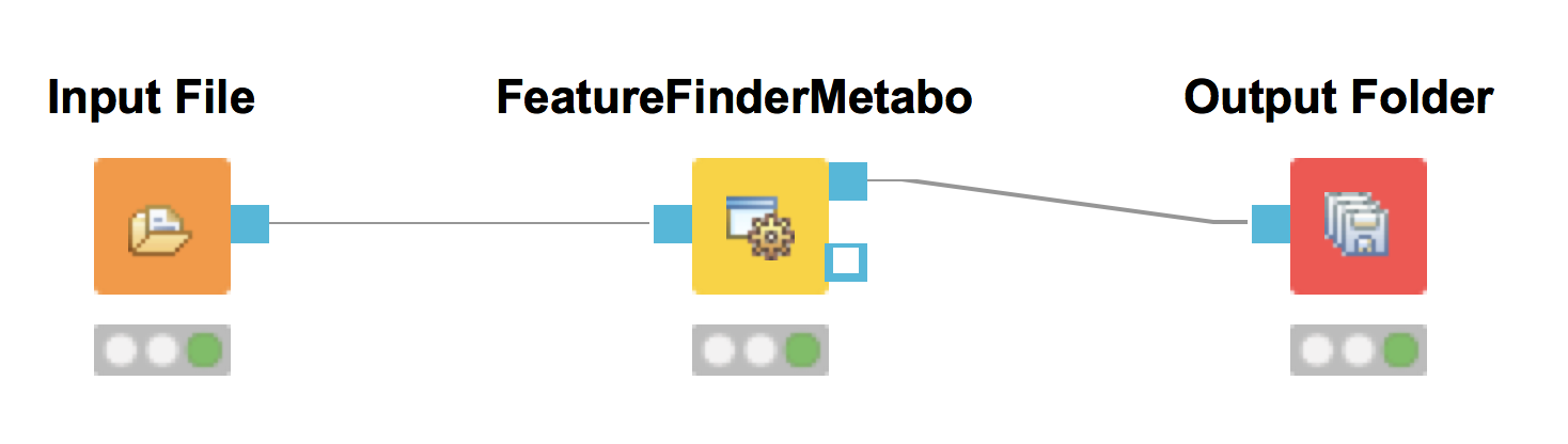
• Connect a Output Folder to the output of the FeatureFinderMetabo (see Fig. 27).

Figure 27: FeatureFinderMetabo workflow

In the following advanced parameters will be highlighted. These parameter can be altered if the Show advanced parameter field in the specific tool is activated.

parameter	value
algorithm→common→chrom_fwhm	8.0
algorithm→mtd→trace_termination_criterion	sample_rate
algorithm→mtd→min_trace_length	3.0
algorithm→mtd→max_trace_length	600.0
algorithm→epd→width_filtering	off
algorithm→ffm→report_convex_hulls	true

The parameters change the behavior of FeatureFinderMetabo as follows:

• chrom_fwhm: The expected chromatographic peak width in seconds.

• trace_termination_criterion: In the first stage FeatureFinderMetabo assembles mass traces with a pre-defined mass accuracy. If this parameter is set to ’outlier’, the extension of a mass trace is stopped after a predefined number of consecutive outliers is found. If this parameter is set to ’sample_rate’, the extension of a mass trace is stopped once the ratio of collected peaks versus visited spectra falls below the ratio given by min_sample_rate.

• min_trace_length: Minimal length of a mass trace in seconds. Choose a small value, if you want to identify low-intensity compounds.

• max_trace_length: Maximal length of a mass trace in seconds. Set this parameter to -1 to disable the filtering by maximal length.

• width_filtering: FeatureFinderMetabo can remove features with unlikely peak widths from the results. If activated it will use the interval provided by the parameters min_fwhm and max_fwhm.

• report_convex_hulls: If set to true, convex hulls including mass traces will be reported for all identified features. This increases the output size considerably.

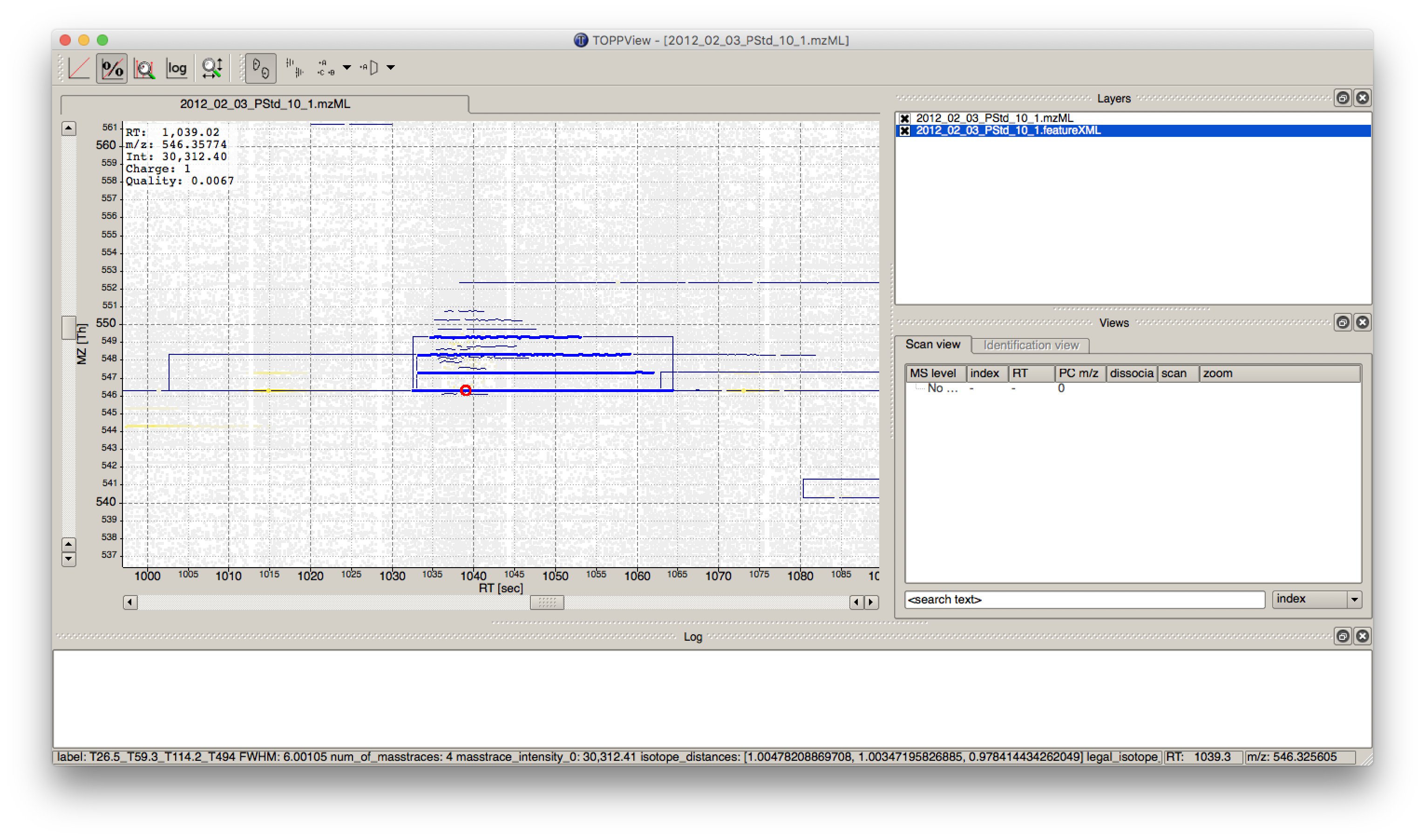
The output file .featureXML can be visualized with TOPPView on top of the used .mzML file - in a so called layer - to look at the identified features.

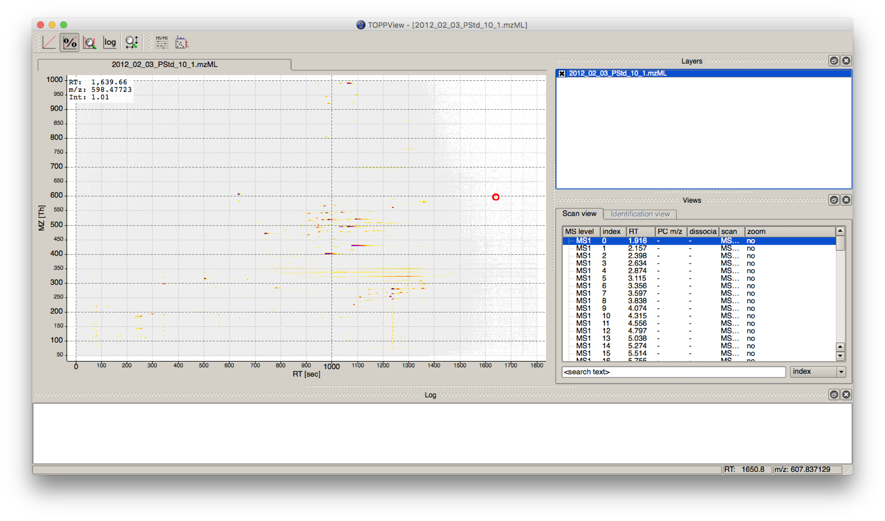
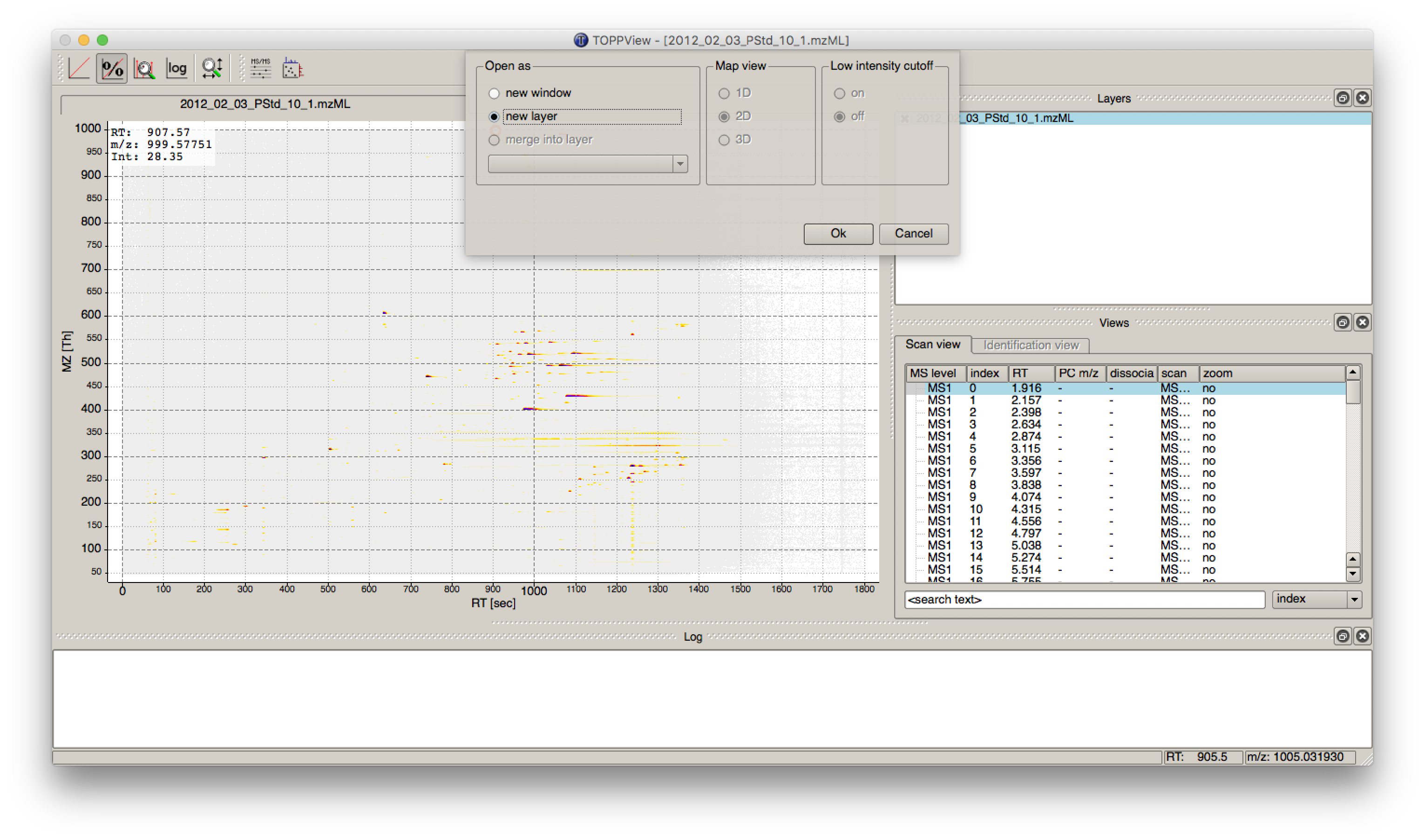
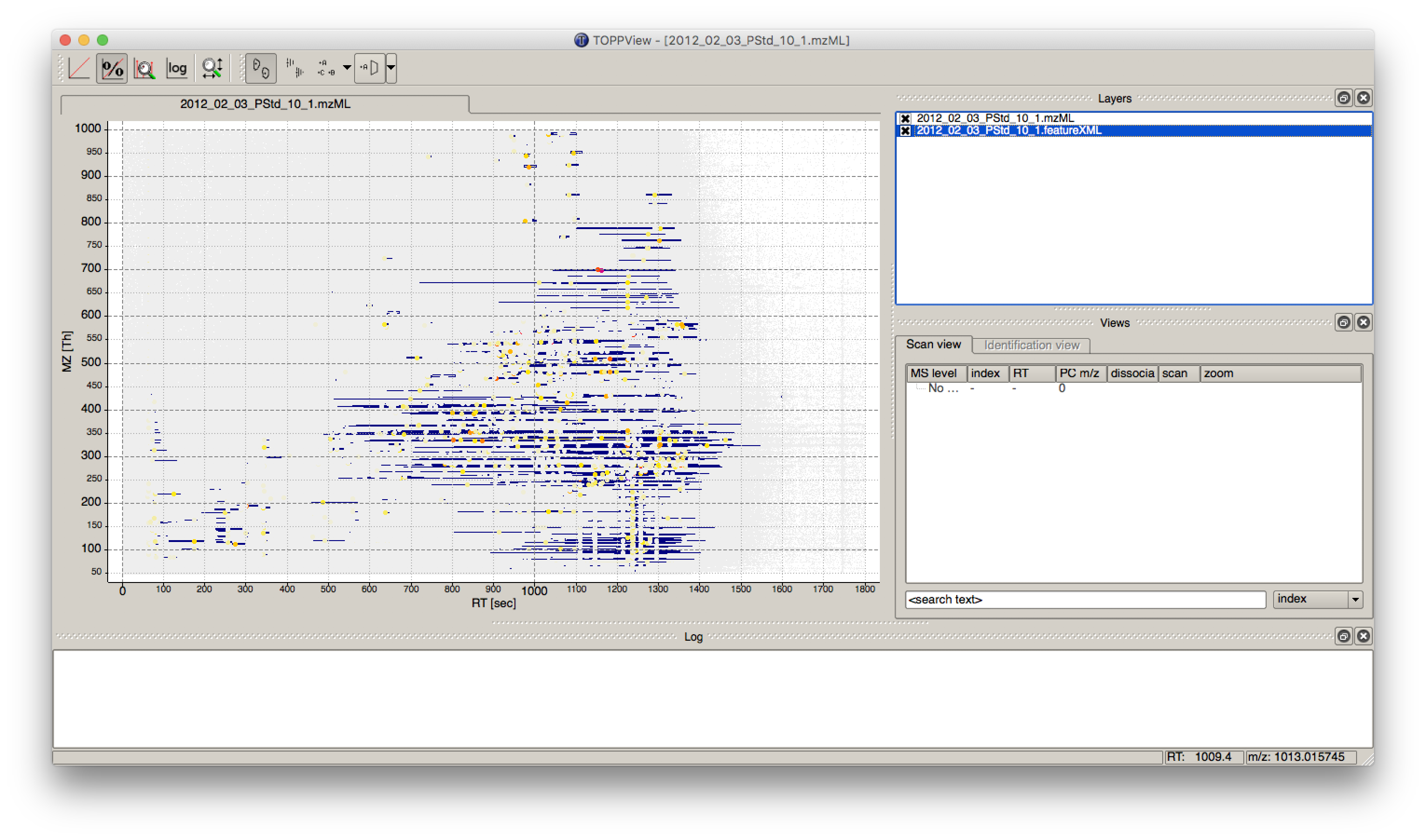
First start TOPPView and open the example .mzML file (see Fig. 28). Afterwards open the .featureXML output as new layer (see Fig. 29). The overlay is depicted in Figure 30. The zoom of the .mzML - .featureXML overlay shows the individual mass traces and the assembly of those in a feature (see Fig. 31).

Figure 28: Opened .mzML in TOPPView

Figure 29: Add new layer in TOPPView

Figure 30: Overlay of the .mzML layer with the .featureXML layer

Figure 31: Zoom of the overlay of the .mzML with the .featureXML layer. Here the individual isotope traces (blue lines) are assembled into a feature here shown as convex hull (rectangular box).

The workflow can be extended for multi-file analysis, here an Input Files node is to be used instead of the File Importer node. In front of the FeatureFinderMetabo, a ZipLoopStart and behind ZipLoopEnd has to be used, since FeatureFinderMetabo will analysis on file to file bases.

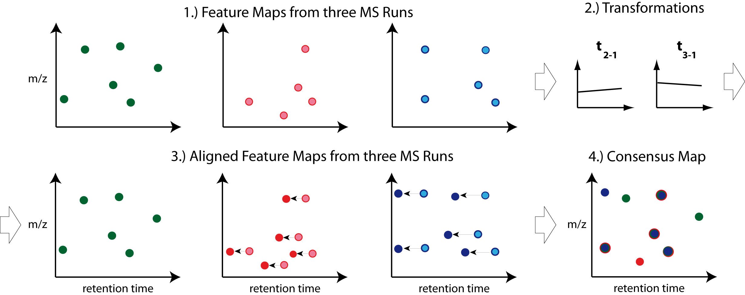
To facilitate the collection of features corresponding to the same compound ion across different samples, an alignment of the samples’ feature maps along retention time is often helpful. In addition to local, small-scale elution differences, one can often see constant retention time shifts across large sections between samples. We can use linear transformations to correct for these large scale retention differences. This brings the majority of corresponding compound ions close to each other. Finding the correct corresponding ions is then faster and easier, as we don’t have to search as far around individual features.

Figure 32: The first feature map is used as a reference to which other maps are aligned. The calculated transformation brings corresponding features into close retention time proximity. Linking of these features form a so-called consensus features of a consensus map.

• After the ZipLoopEnd node, add a MapAlignerPoseClustering node (Community Nodes>OpenMS>Map Alignment), set its Output Type to featureXML, and adjust the following settings:

parameter	value
algorithm → max_num_peaks_considered	−1
algorithm → superimposer → mz_pair_max_distance	0.005
algorithm → superimposer → num_used_points	10000
algorithm → pairfinder → distance_RT → max_difference	20.0
algorithm → pairfinder → distance_MZ → max_difference	20.0
algorithm → pairfinder → distance_MZ → unit	ppm

MapAlignerPoseClustering provides an algorithm to align the retention time scales of multiple input files, correcting shifts and distortions between them. Retention time adjustment may be necessary to correct for chromatography differences e.g. before data from multiple LC-MS runs can be combined (feature linking). The alignment algorithm implemented here is the pose clustering algorithm.

The parameters change the behavior of MapAlignerPoseClustering as follows:

• max_num_peaks_considered: The maximal number of peaks/features to be considered per map. To use all, set this parameter to -1.

• mz_pair_max_distance: Maximum of m/z deviation of corresponding elements in different maps. This condition applies to the pairs considered in hashing.

• num_used_points: Maximum number of elements considered in each map (selected by intensity). Use a smaller number to reduce the running time and to disregard weak signals during alignment.

• distance_RT → max_difference: Features that have a larger RT difference will never be paired.

• distance_MZ →max_difference: Features that have a larger m/z difference will never be paired.

• distance_MZ →unit: Unit used for the parameter distance_MZ max_difference, either Da or ppm.

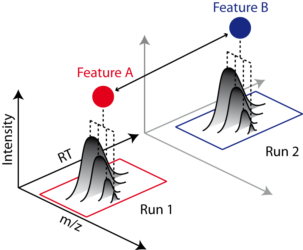
The next step after retention time correction is the grouping of corresponding features in multiple samples. In contrast to the previous alignment, we assume no linear relations of features across samples. The used method is tolerant against local swaps in elution order.

Figure 33: Features A and B correspond to the same analyte. The linking of features between runs (indicated by an arrow) allows comparing feature intensities.

• After the MapAlignerPoseClustering node, add a FeatureLinkerUnlabeledQT node (Community Nodes > OpenMS>Map Alignment) and adjust the following settings:

  |parameter|value| |:————|:——–| |algorithm → distance_RT → max_difference|40| |algorithm → distance_MZ → max_difference|20| |algorithm → distance_MZ → unit|ppm|

  The parameters change the behavior of FeatureLinkerUnlabeledQT as follows (similar to the parameters we adjusted for MapAlignerPoseClustering):

  • distance_RT → max_difference: Features that have a larger RT difference will never be paired.

  • distance_MZ → max_difference: Features that have a larger m/z difference will never be paired.

  • distance_MZ → unit: Unit used for the parameter distance_MZ max_difference, either Da or ppm.

• After the FeatureLinkerUnlabeledQT node, add a TextExporter node (Community Nodes > OpenMS > File Handling).

• Add an Output Folder node and configure it with an output directory where you want to store the resulting files.

• Run the pipeline and inspect the output.

Figure 34: Label-free quantification workflow for metabolites.

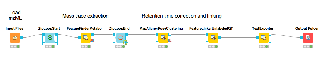
You should find a single, tab-separated file containing the information on where metabolites were found and with which intensities. You can also add Output Folder nodes at different stages of the workflow and inspect the intermediate results (e.g., identified metabolite features for each input map). The complete workflow can be seen in Figure 34. In the following section we will try to identify those metabolites.

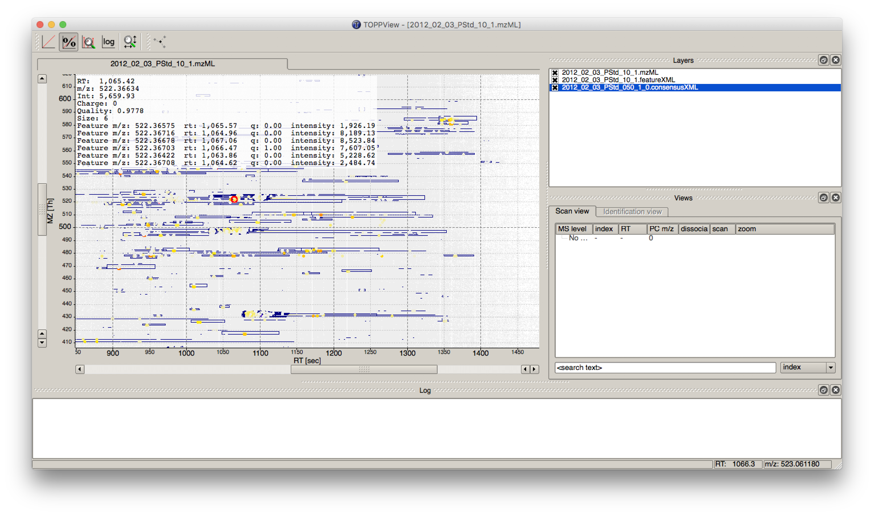
The FeatureLinkerUnlabeledQT output can be visualized in TOPPView on top of the input and output of the FeatureFinderMetabo (see Fig 35).

Figure 35: Visualization of .consensusXML output over the .mzML and .featureXML ’layer’.

Basic metabolite identification

At the current state we found several metabolites in the individual maps but so far don’t know what they are. To identify metabolites, OpenMS provides multiple tools, including search by mass: the AccurateMassSearch node searches observed masses against the Human Metabolome Database (HMDB)[1]^, [2]^, [3]. We start with the workflow from the previous section (see Figure 34).

• Add a FileConverter node (Community Nodes > OpenMS > File Handling) and connect the output of the FeatureLinkerUnlabeledQT to the incoming port.

• Open the Configure dialog of the FileConverter node and select the tab OutputTypes. In the drop down list for FileConverter.1.out select featureXML.

• Add an AccurateMassSearch node (Community Nodes > OpenMS > Utilities) and connect the output of the FileConverter node to the first port of the AccurateMassSearch node.

• Add four File Importer nodes and configure them with the following files:

  • Example_Data▸Metabolomics▸databases▸PositiveAdducts.tsv This file specifies the list of adducts that are considered in the positive mode. Each line contains the formula and charge of an adduct separated by a semicolon (e.g. M+H;1+). The mass of the adduct is calculated automatically.

  • Example_Data▸Metabolomics▸databases▸NegativeAdducts.tsv This file specifies the list of adducts that are considered in the negative mode analogous to the positive mode.

  • Example_Data▸Metabolomics▸databases▸HMDBMappingFile.tsv This file contains information from a metabolite database in this case from HMDB. It has three (or more) tab-separated columns: mass, formula, and identifier(s). This allows for an efficient search by mass.

  • Example_Data▸Metabolomics▸databases▸HMDB2StructMapping.tsv This file contains additional information about the identifiers in the mapping file. It has four tab-separated columns that contain the identifier, name, SMILES, and INCHI. These will be included in the result file. The identifiers in this file must match the identifiers in the HMDBMappingFile.tsv.

• In the same order as they are given above connect them to the remaining input ports of the AccurateMassSearch node.

• Add an Output Folder node and connect the first output port of the AccurateMassSearch node to the Output Folder node.

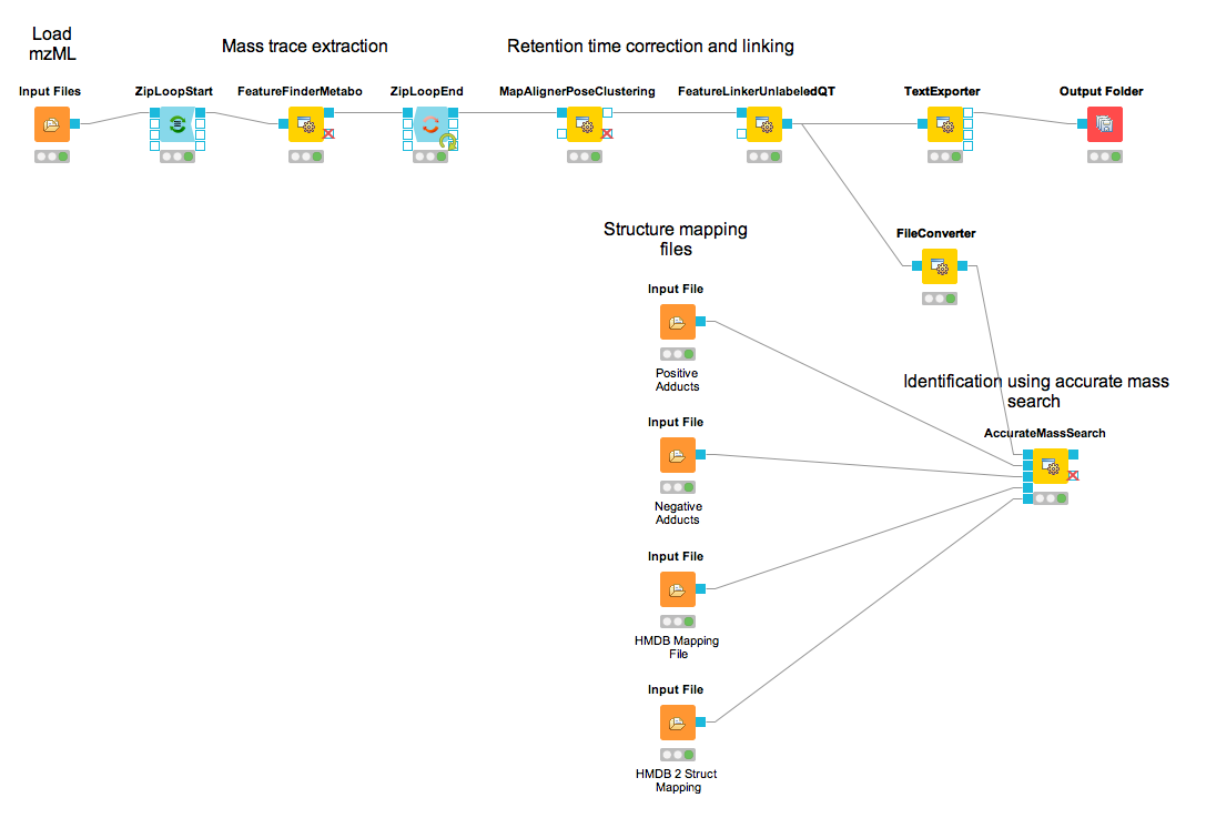
The result of the AccurateMassSearch node is in the mzTab format[4] so you can easily open it in a text editor or import it into Excel or KNIME, which we will do in the next section. The complete workflow from this section is shown in Figure 36.

Figure 36: Label-free quantification and identification workflow for metabolites.

Convert your data into a KNIME table

The result from the TextExporter node as well as the result from the AccurateMassSearch node are files while standard KNIME nodes display and process only KNIME tables. To convert these files into KNIME tables we need two different nodes. For the AccurateMassSearch results, we use the MzTabReader node (Community Nodes > OpenMS > Conversion > mzTab) and its Small Molecule Section port. For the result of the TextExporter, we use the ConsensusTextReader (Community Nodes > OpenMS > Conversion). 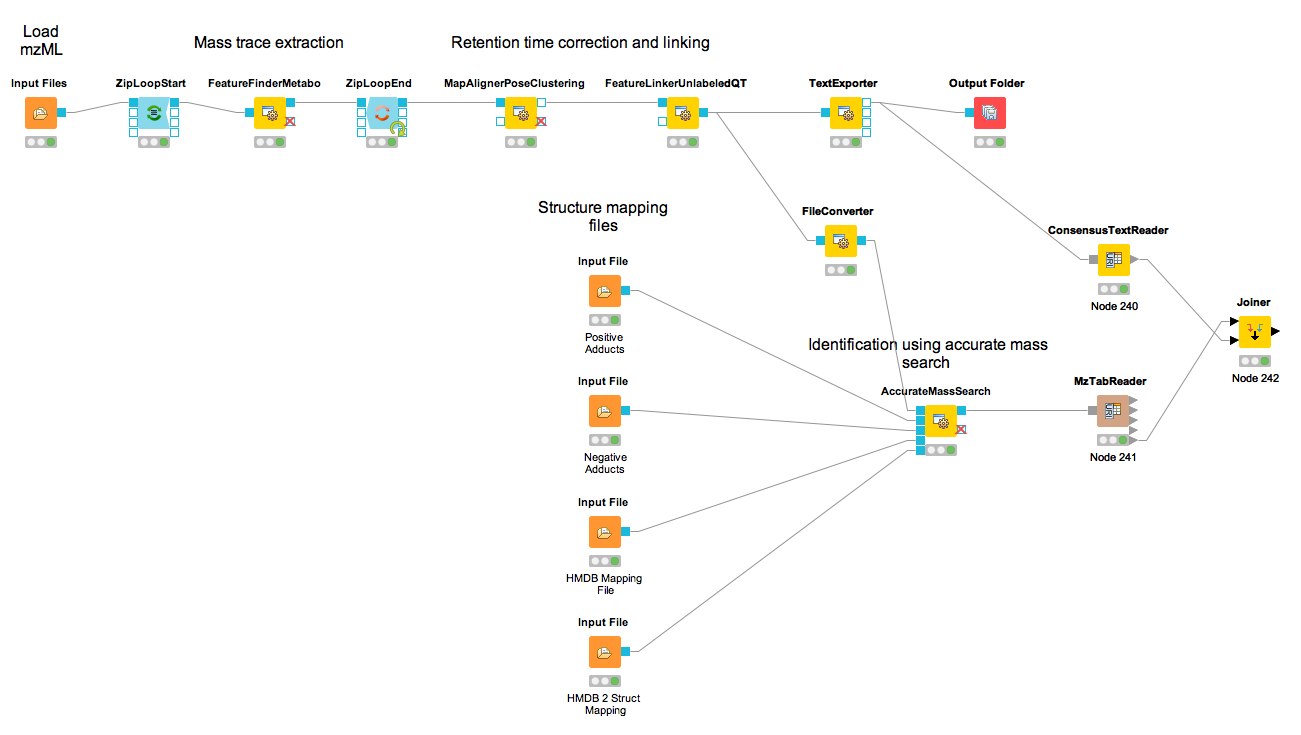When executed, both nodes will import the OpenMS files and provide access to the data as KNIME tables. The retention time values are exported as a list using the MzTabReader based on the current PSI-Standard. This has to be parsed using the SplitCollectionColumn, which outputs a ”Split Value 1” based on the first entry in the rention time list, which has to be renamed to retention time using the ColumnRename. You can now combine both tables using the Joiner node (Manipulation > Column > Split & Combine) and configure it to match the m/z and retention time values of the respective tables. The full workflow is shown in Figure 37.

Figure 37: Label-free quantification and identification workflow for metabolites that loads the results into KNIME and joins the tables.

Adduct grouping

Metabolites commonly co-elute as ions with different adducts (e.g., glutathione+H, glutathione+Na) or with charge-neutral modifications (e.g., water loss). Grouping such related ions allows to leverage information across features. For example, a low intensity, single trace feature could still be assigned a charge and adduct due to a matching high-quality feature. Several OpenMS tools, such as AccurateMassSearch, can use this information to, for example, narrow down candidates for identification.

For this grouping task, we provide the MetaboliteAdductDecharger node. Its method explores the combinatorial space of all adduct combinations in a charge range for optimal explanations. Using defined adduct probabilities, it assigns co-eluting features having suitable mass shifts and charges those adduct combinations which maximize overall ion probabilities.

The tool works natively with featureXML data, allowing the use of reported convex hulls. On such a single-sample level, co-elution settings can be chosen more stringently, as ionization-based adducts should not influence the elution time: Instead, elution differences of related ions should be due to slightly differently estimated times for their feature centroids.

Alternatively, consensusXML data from feature linking can be converted for use, though with less chromatographic information. Here, the elution time averaging for features linked across samples, motivates wider co-elution tolerances.

The two main tool outputs are a consensusXML file with compound groups of related input ions, and a featureXML containing the input file but annotated with inferred adduct information and charges.

Options to respect or replace ion charges or adducts allow for example:

• Heuristic but faster, iterative adduct grouping(MetaboliteAdductDecharger → MetaboliteFeatureDeconvolution → q_try set to “feature”) by chaining multiple MetaboliteAdductDecharger nodes with growing adduct sets, charge ranges or otherwise relaxed tolerances.

• More specific feature linking (FeatureLinkerUnlabeledQT → algorithm → ignore_adduct set to “false”)

Figure 38: Metabolite Adduct Decharger adduct grouping workflow.

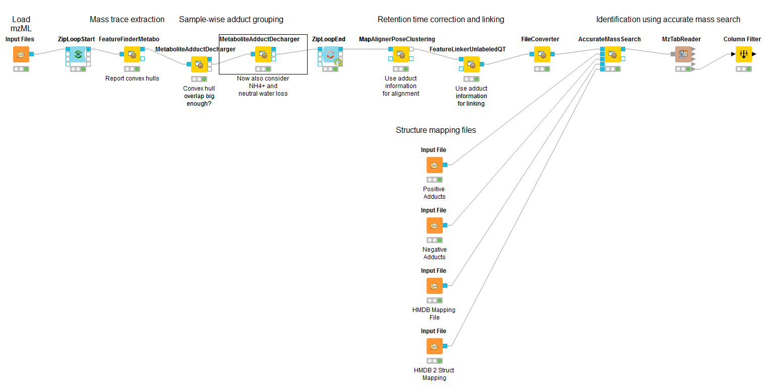
Task

A modified metabolomics workflow with exemplary MetaboliteAdductDecharger use and parameters is provided in Workflows▸MetaboliteAdductGrouping.knwf. Run the workflow, inspect tool outputs and compare AccurateMassSearch results with and without adduct grouping.

Visualizing data

Now that you have your data in KNIME you should try to get a feeling for the capabilities of KNIME.

Task

Check out the Molecule Type Cast node (Chemistry > Translators) together with subsequent cheminformatics nodes (e.g. RDKit From Molecule(Community Nodes > RDKit > Converters)) to render the structural formula contained in the result table.

Task

Have a look at the Column Filter node to reduce the table to the interesting columns, e.g., only the Ids, chemical formula, and intensities.

Task

Try to compute and visualize the m/z and retention time error of the different feature elements (from the input maps) of each consensus feature. Hint: A nicely configured Math Formula (Multi Column) node should suffice.

Spectral library search

Identifying metabolites using only the accurate mass may lead to ambiguous results. In practice, additional information (e.g. the retention time) is used to further narrow down potential candidates. Apart from MS1-based features, tandem mass spectra (MS2) of metabolites provide additional information. In this part of the tutorial, we take a look on how metabolite spectra can be identified using a library of previously identified spectra.

Because these libraries tend to be large we don’t distribute them with OpenMS.

Task

Construct the workflow as shown in Fig. 39. Use the file ExampleData▸Metabolomics▸datasets▸MetaboliteIDSpectraDBpositive.mzML as input for your workflow. You can use the spectral library from ExampleData▸Metabolomics▸databases▸MetaboliteSpectralDB.mzML as second input. The first input file contains tandem spectra that are identified by the MetaboliteSpectralMatcher. The resulting mzTab file is read back into a KNIME table The retention time values are exported as a list based on the current PSI-Standard. This has to be parsed using the SplitCollectionColumn, which outputs a ”Split Value 1” based on the first entry in the rention time list, which has to be renamed to retention time using the ColumnRename before it is stored in an Excel table. Make sure that you connect the MzTabReader port corresponding to the Small Molecule Section to the Excel writer (XLS). Please select the ”add column headers” option in the Excel writer (XLS)).

Figure 39: Spectral library identification workflow.

Run the workflow and inspect the output.

Manual validation

In metabolomics, matches between tandem spectra and spectral libraries are manually validated. Several commercial and free online resources exist which help in that task. Some examples are:

• mzCloud contains only spectra from Thermo Orbitrap instruments. The webpage requires Microsoft Silverlight which currently does not work in modern browsers (see the following link.

• MassBank North America (MoNA) has spectra from different instruments but falls short in number of spectra (compared to Metlin and mzCloud). See the following link.

• METLIN includes 961,829 molecules ranging from lipids, steroids, metabolites, small peptides, carbohydrates, exogenous drugs and toxicants. In total over 14,000 metabolites.

Here, we will use METLIN to manually validate metabolites.

Task

Check in the .xlsx output from the Excel writer (XLS) if you can find glutathione. Use the retention time column to find the spectrum in the mzML file. Here open the file in the Example_Data▸Metabolomics▸datasets▸MetaboliteIDSpectraDBpositive.mzML in TOPPView. The MSMS spectrum with the retention time of 67.6 s is used as example. The spectrum can be selected based on the retention time in the scan view window. Therefore the MS1 spectrum with the retention time of 66.9 s has to be double clicked and the MSMS spectra recorded in this time frame will show up. Select the tandem spectrum of Glutathione, but do not close TOPPView, yet.

Figure 40: Tandem spectrum of glutathione. Visualized in TOPPView.

Task

On the METLIN homepage search for Name Glutathione using the Advanced Search. See the link. Note that free registration is required. Which collision energy (and polarity) gives the best (visual) match to your experimental spectrum in TOPPView? Here you can compare the fragmentation patterns in both spectra shown by the Intensity or relative Intensity, the m/z of a peak and the distance between peaks. Each distance between two peaks corresponds to a fragment of elemental composition (e.g., NH2 with the charge of one would have mass of two peaks of 16.023 Th).

Figure 41: Tandem spectrum of glutathione. Visualized in Metlin. Note that several fragment spectra from varying collision energies are available.

De novo identification

Another method for MS2 spectra-based metabolite identification is de novo identification. This approach can be used in addition to the other methods (accurate mass search, spectral library search) or individually if no spectral library is available. In this part of the tutorial, we discuss how metabolite spectra can be identified using de novo tools. To this end, the tools SIRIUS and CSI:FingerID ([5]^, [6]^, [7]) were integrated in the OpenMS Framework as SiriusAdapter. SIRIUS uses isotope pattern analysis to detect the molecular formula and further analyses the fragmentation pattern of a compound using fragmentation trees. CSI:FingerID is a method for searching a fingerprint of a small molecule (metabolite) in a molecular structure database. The node SiriusAdapter is able to work in different modes depending on the provided input.

• Input: mzML - SiriusAdapter will search all MS2 spectra in a map.

• Input: mzML, featureXML (FeatureFinderMetabo) - SiriusAdapter can use the provided feature information to reduce the search space to valid features with MS2 spectra. Additionally it can use the isotopic trace information.

• Input: mzML, featureXML (FeatureFinderMetabo / MetaboliteAdductDecharger / AccurateMassSearch) - SiriusAdapter can use the feature information as mentioned above together with feature adduct information from adduct grouping or previous identification.

By using a mzML and featureXML, SIRIUS gains a lot of additional information by using the OpenMS tools for preprocessing.

Task

Construct the workflow as shown in Fig. 42. Example_Data▸Metabolomics▸datasets Use the file MetaboliteDeNovoID.mzML as input for your workflow.

Below we show an example workflow for de novo identification (Fig. 42). Here, the node FeatureFinderMetabo is used for feature detection to annotate analytes in mz, rt, intensity and charge. This is followed by adduct grouping, trying to asses possible adducts based on the feature space using the MetaboliteAdductDecharger. In addition, the HighResPrecursorMassCorrector can use the newly generated feature information to map MS2 spectra, which were measured on one of the isotope traces to the monoisotopic precursor. This helps with feature mapping and analyte identification in the SiriusAdapter due to the usage of additional MS2 spectra that belong to a specific feature.

Figure 42: De novo identification workflow

Run the workflow and inspect the output.

The output consists of two mzTab files and an internal .ms file. One mzTab for SIRIUS and the other for the CSI:FingerID. These provide information about the chemical formula, adduct and the possible compound structure. The information is referenced to the spectrum used in the analysis. Additional information can be extracted from the SiriusAdapter by setting an ”out_workspace_directory”. Here the SIRIUS workspace will be provided after the calculation has finished. This workspace contains information about annotated fragments for each successfully explained compound.

Downstream data analysis and reporting

In this part of the metabolomics session we take a look at more advanced downstream analysis and the use of the statistical programming language R. As laid out in the introduction we try to detect a set of spike-in compounds against a complex blood background. As there are many ways to perform this type of analysis we provide a complete workflow.

Task

Import the workflow from Workflows ► metaboliteID.knwf in KNIME: File > Import KNIME Workflow…

The section below will guide you in your understanding of the different parts of the workflow. Once you understood the workflow you should play around and be creative. Maybe create a novel visualization in KNIME or R? Do some more elaborate statistical analysis? Note that some basic R knowledge is required to fully understand the processing in R Snippet nodes.

Signal processing and data preparation for identification

The following part is analogous to what you did for the simple metabolomics pipeline.

Data preparation for quantification

The first part is identical to what you did for the simple metabolomics pipeline. Additionally, we convert zero intensities into NA values and remove all rows that contain at least one NA value from the analysis. We do this using a very simple R Snippet and subsequent Missing Value filter node.

Task

Inspect the R Snippet by double-clicking on it. The KNIME table that is passed to an R Snippet node is available in R as a data.frame named knime.in. The result of this node will be read from the data.frame knime.out after the script finishes. Try to understand and evaluate parts of the script (Eval Selection). In this dialog you can also print intermediary results using for example the R command head(knime.in) or cat(knime.in) to the Console pane.

Statistical analysis

After we linked features across all maps, we want to identify features that are significantly deregulated between the two conditions. We will first scale and normalize the data, then perform a t-test, and finally correct the obtained p-values for multiple testing using Benjamini-Hochberg. All of these steps will be carried out in individual R Snippet nodes.

• Double-click on the first R Snippet node labeled ”log scaling” to open the R Snippet dialog. In the middle you will see a short R script that performs the log scaling. To perform the log scaling we use a so-called regular expression (grepl) to select all columns containing the intensities in the six maps and take the log2 logarithm.

• The output of the log scaling node is also used to draw a boxplot that can be used to examine the structure of the data. Since we only want to plot the intensities in the different maps (and not m/z or rt) we first use a Column Filter node to keep only the columns that contain the intensities. We connect the resulting table to a Box Plot node which draws one box for every column in the input table. Right-click and select View: Box Plot

• The median normalization is performed in a similar way to the log scaling. First we calculate the median intensity for each intensity column, then we subtract the median from every intensity.

• Open the Box Plot connected to the normalization node and compare it to the box plot connected to the log scaling node to examine the effect of the median normalization.

• To perform the t-test we defined the two groups we want to compare. Finally we save the p-values and fold-changes in two new columns named p-value and FC.

• The Numeric Row Splitter is used to filter less interesting parts of the data. In this case we only keep columns where the fold-change is ≥ 2.

• We adjust the p-values for multiple testing using Benjamini-Hochberg and keep all consensus features with a q-value ≤ 0.01 (i.e. we target a false-discovery rate of 1%).

Interactive visualization

KNIME supports multiple nodes for interactive visualization with interrelated output. The nodes used in this part of the workflow exemplify this concept. They further demonstrate how figures with data dependent customization can be easily realized using basic KNIME nodes. Several simple operations are concatenated in order to enable an interactive volcano plot.

• We first log-transform fold changes and p-values in the R Snippet node. We then append columns noting interesting features (concerning fold change and p-value).

• With this information, we can use various Manager nodes (Views > Property) to emphasize interesting data points. The configuration dialogs allow us to select columns to change color, shape or size of data points dependent on the column values.

• The Scatter Plot node (from the Views repository) enables interactive visualization of the logarithmized values as a volcano plot: the log-transformed values can be chosen in the ‘Column Selection’ tab of the plot view. Data points can be selected in the plot and highlighted via the menu option. The highlighting transfers to all other interactive nodes connected to the same data table. In our case, selection and the highlighting will also occur in the Interactive Table node (from the Views repository).

• Output of the interactive table can then be filtered via the ”HiLite” menu tab. For example, we could restrict shown rows to points highlighted in the volcano plot.

Task

Inspect the nodes of this section. Customize your visualization and possibly try to visualize other aspects of your data.

Advanced visualization

R Dependencies: This section requires that the R packages ggplot2 and ggfortify are both installed. ggplot2 is part of the KNIME R Statistics Integration (Windows Binaries) which should already be installed via the full KNIME installer, ggfortify however is not. In case that you use an R installation where one or both of them are not yet installed, add an R Snippet node and double-click to configure. In the R Script text editor, enter the following code:

#Include the next line if you also have to install ggplot2:   
install.packages("ggplot2")
 
#Include the following lines to install ggfortify:  
install.packages("ggfortify")
 
library(ggplot2) 
library(ggfortify)

You can remove the:

install.packages

commands once it was successfully installed.

Even though the basic capabilities for (interactive) plots in KNIME are valuable for initial data exploration, professional looking depiction of analysis results often relies on dedicated plotting libraries. The statistics language R supports the addition of a large variety of packages, including packages providing extensive plotting capabilities. This part of the workflow shows how to use R nodes in KNIME to visualize more advanced figures. Specifically, we make use of different plotting packages to realize heatmaps.

• The used RView (Table) nodes combine the possibility to write R snippet code with visualization capabilities inside KNIME. Resulting images can be looked at in the output RView, or saved via the Image Writer (Port) node.

• The heatmap nodes make use of the gplots libary, which is by default part of the R Windows binaries (for full KNIME version 3.1.1 or higher). We again use regular expressions to extract all measured intensity columns for plotting. For clarity, feature names are only shown in the heatmap after filtering by fold changes.

Data preparation for reporting

Following the identification, quantification and statistical analysis our data is merged and formatted for reporting. First we want to discard our normalized and logarithmized intensity values in favor of the original ones. To this end we first remove the intensity columns (Column Filter) and add the original intensities back (Joiner). For that, we use an Inner Join 2 with the Joiner node. In the dialog of the node, we add two entries for the Joining Columns and for the first column we pick retention_time from the top input (i.e. the AccurateMassSearch output) and rt_cf (the retention time of the consensus features) for the bottom input (the result from the quantification). For the second column you should choose exp_mass_to_charge and mz_cf respectively to make the joining unique. Note that the workflow needs to be executed up to the previous nodes for the possible selections of columns to appear.

Figure 43: Data preparation for reporting

Question

What happens if we use a Left Outer Join, Right Outer Join or Full Outer Join instead of the Inner Join?

Task

Inspect the output of the join operation after the Molecule Type Cast and RDKit molecular structure generation.

While all relevant information is now contained in our table the presentation could be improved. Currently, we have several rows corresponding to a single consensus feature (=linked feature) but with different, alternative identifications. It would be more convenient to have only one row for each consensus feature with all accurate mass identifications added as additional columns. To this end, we use the Column to Grid node that flattens several rows with the same consensus number into a single one. Note that we have to specify the maximum number of columns in the grid so we set this to a large value (e.g. 100). We finally export the data to an Excel file (XLS Writer).

References

[1]

D. S. Wishart, D. Tzur, C. Knox, et al., HMDB: the Human Metabolome Database, Nucleic Acids Res 35(Database issue), D521–6 (Jan 2007), doi:10.1093/nar/gkl923. 69

[2]

D. S. Wishart, C. Knox, A. C. Guo, et al., HMDB: a knowledgebase for the human metabolome, Nucleic Acids Res 37(Database issue), D603–10 (Jan 2009), doi: 10.1093/nar/gkn810. 69

[3]

D. S. Wishart, T. Jewison, A. C. Guo, M. Wilson, C. Knox, et al., HMDB 3.0–The Human Metabolome Database in 2013, Nucleic Acids Res 41(Database issue),D801–7 (Jan 2013), doi:10.1093/nar/gks1065. 69

[4]

J. Griss, A. R. Jones, T. Sachsenberg, M. Walzer, L. Gatto, J. Hartler, G. G. Thallinger, R. M. Salek, C. Steinbeck, N. Neuhauser, J. Cox, S. Neumann, J. Fan, F. Reisinger, Q.-W. Xu, N. Del Toro, Y. Perez-Riverol, F. Ghali, N. Bandeira, I. Xenarios, O. Kohlbacher, J. A. Vizcaino, and H. Hermjakob, The mzTab Data Exchange Format: communicating MS-based proteomics and metabolomics experimental results to a wider audience, Mol Cell Proteomics (Jun 2014), doi:10.1074/mcp.O113.036681. 69

[5]

S. Böcker, M. C. Letzel, Z. Lipták, and A. Pervukhin, SIRIUS: Decomposing isotope patterns for metabolite identification, Bioinformatics 25(2), 218–224 (2009), doi:10.1093/bioinformatics/btn603. 75

[6]

S. Böcker and K. Dührkop, Fragmentation trees reloaded, J. Cheminform. 8(1), 1–26 (2016), doi:10.1186/s13321-016-0116-8. 75

[7]

K. Dührkop, H. Shen, M. Meusel, J. Rousu, and S. Böcker, Searching molecular structure databases with tandem mass spectra using CSI:FingerID, Proc. Natl. Acad. Sci. 112(41), 12580–12585 (oct 2015), doi:10.1073/pnas.1509788112. 75