Views in TOPPView
TOPPView offers three types of views – a 1D view for spectra, a 2D view for peak maps and feature maps, and a 3D view for peak maps. All three views can be freely configured to suit the individual needs of the user.
Action Modes and Their Uses
All three views share a similar interface. Three action modes are supported – one for translation, one for zooming and one for measuring:
Translate mode
It is activated by default
Move the mouse while holding the mouse button down to translate the current view
Arrow keys can be used to translate the view without entering translate mode (in 1D-View you can additionally use Shift to jump to the next peak)
Zoom mode
All previous zoom levels are stored in a zoom history. The zoom history can be traversed using CTRL + +/CTRL + - or the mouse wheel (scroll up and down)
Zooming into the data:
Mark an area in the current view with your mouse, while holding the left mouse button plus the CTRL key to zoom to this area.
You can also use your mouse wheel to traverse the zoom history.
If you have reached the end of the history, keep on pressing CTRL + + or scroll up, the current area will be enlarged by a factor of
1.25.
Pressing Backspace resets the zoom and zoom history.
Measure mode
It is activated using SHIFT.
Press the left mouse button down while a peak is selected and drag the mouse to another peak to measure the distance between peaks.
This mode is implemented in the 1D and 2D mode.
1D View
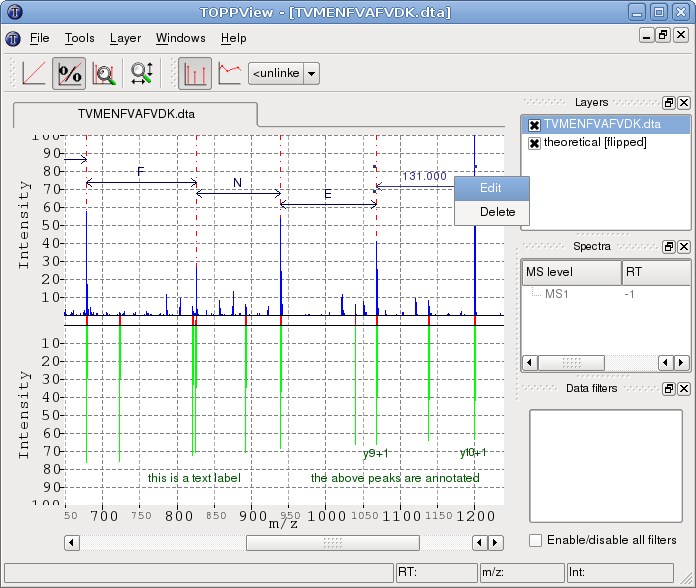
The 1D view is used to display raw spectra or peak spectra. Raw data is displayed using a continuous line. Peak data is displayed using one stick per peak. The color used for drawing the lines can be set for each layer individually. The 1D view offers a mirror mode, where the window is vertically divided in halves and individual layers can be displayed either above or below the “mirror” axis in order to facilitate quick visual comparison of spectra. When a mirror view is active, it is possible to perform a spectrum alignment of a spectrum in the upper and one in the lower half, respectively. Moreover, spectra can be annotated manually. Currently, distance annotations between peaks, peak annotations and simple text labels are provided.
The following example image shows a 1D view in mirror mode. A theoretical spectrum (lower half) has been generated using the theoretical spectrum generator (Tools > Generate theoretical spectrum). The mirror mode has been activated by right-clicking the layer containing the theoretical spectrum and selecting Flip downward from the layer context menu. A spectrum alignment between the two spectra has been performed (Tools > Align spectra). It is visualized by the red lines connecting aligned peaks and can be reset through the context menu. Moreover, in the example, several distances between abundant peaks have been measured and subsequently replaced by their corresponding amino acid residue code. This is done by right-clicking a distance annotation and selecting Edit from the context menu. Additionally, peak annotations and text labels have been added by right-clicking peaks and selecting Add peak annotation or by right clicking anywhere and selecting Add Label, respectively. Multiple annotations can be selected by holding down the CTRL key while clicking them. They can be moved around by dragging the mouse and deleted by pressing DEL.
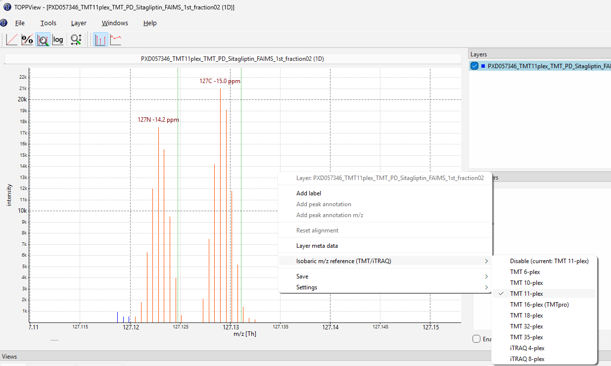
When inspecting fragment (MS2) spectra of isobarically labeled samples, the 1D view can overlay the theoretical
reporter-ion m/z positions of a chosen labeling method. Right-click the spectrum and pick a method from the
Isobaric m/z reference (TMT/iTRAQ) submenu; the supported methods include TMT 6-, 10-, 11-, 16-, 18-, 32- and
35-plex as well as iTRAQ 4- and 8-plex. For every channel a vertical reference line is drawn at its expected m/z: a
solid green line when a matching peak is found in the spectrum, and a dashed grey line labeled with the channel name
when the channel is missing. Matched peaks are highlighted and annotated with the measured mass deviation in ppm. The
overlay works for both profile and centroided spectra and is updated automatically as you navigate between spectra.
Choose Disable from the same submenu to remove it again.
The following example shows a TMT 11-plex fragment spectrum with the Isobaric m/z reference (TMT/iTRAQ) submenu open.
Matched reporter ions are drawn in orange and labeled with their channel name and mass deviation (e.g. 127N -14.2 ppm,
127C -15.0 ppm):
Through the context menu: of the 1D view you can:
View/edit meta data.
Save the current layer data.
Change display settings.
Add peak annotations or arbitrary text labels.
Reset a performed alignment.
Overlay theoretical isobaric (TMT/iTRAQ) reporter-ion
m/zreferences via the Isobaric m/z reference (TMT/iTRAQ) submenu.
2D View
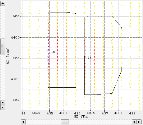
The 2D view is used to display peak maps and feature maps in a top-down view with color-coded intensities. Peaks and feature centroids are displayed as dots. For features, also the overall convex hull and the convex hulls of individual mass traces can be displayed. The color gradient used to encode for peak and feature intensities can be set for each layer individually.
The following example image shows a small section of a peak map and the detected features in a second layer.
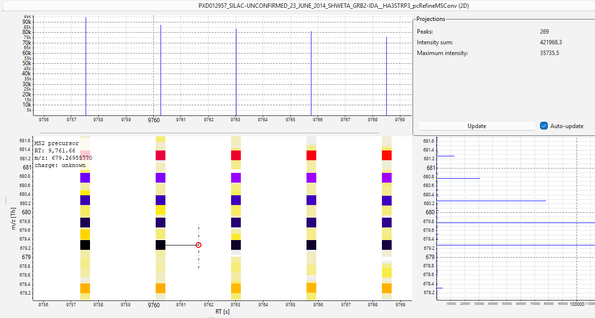
In addition to the normal top-down view, the 2D view can display the projections of the data to the m/z and RT axis.
This feature is mainly used to assess the quality of a feature without opening the data region in 3D view.
When you move the mouse over the 2D view, the data point closest to the cursor is highlighted with a red circle and its
coordinates (RT, m/z and intensity) are shown in the upper left corner of the view.
If the display of MS/MS precursors is enabled (see Display Modes and View Options, option 2D (Peaks)), the
precursor of each fragment (MS2) scan is marked as well: a rhombus at the precursor position in the preceding survey
(MS1) scan, a line connecting it to the retention time of the fragment scan, and – if isolation window information is
available – a dashed line indicating the isolated m/z range. Precursor markers are treated just like peaks when
highlighting: moving the mouse over a precursor marker highlights it and shows the precursor’s RT, m/z and charge in
the upper left corner.
The following example shows a fragment scan precursor (red circle) with its connecting line and isolation window (dashed
line); the upper left corner displays the precursor’s RT, m/z and charge:
Through the context menu: of the 2D view you can:
View/edit meta data
View survey/fragment scans in 1D view
View survey/fragment scans meta data
View the currently selected area in 3D view
Save the current layer data
Change display settings
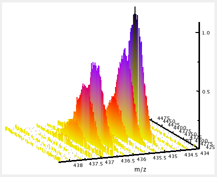
3D View
The 3D view can only display peak maps. Its primary use is the closer inspection of a small region of the map, e.g. a single feature. In the 3D view slight intensity differences are easier to recognize than in the 2D view. The color gradient used to encode peak intensities, the width of the lines and the coloring mode of the peaks can be set for each layer individually.
The following example image shows a small region of a peak map:
Through the context menu: of the 3D view you can:
View/edit meta data.
Save the current layer data.
Change display setting.