Quality control
Introduction
In this chapter, we will build on an existing workflow with OpenMS / KNIME to add some quality control (QC). We will utilize the qcML tools in OpenMS to create a file with which we can collect different measures of quality to the mass spectrometry runs themselves and the applied analysis. The file also serves the means of visually reporting on the collected quality measures and later storage along the other analysis result files. We will, step-by-step, extend the label-free quantitation workflow from section 3 with QC functions and thereby enrich each time the report given by the qcML file. But first, to make sure you get the most of this tutorial section, a little primer on how we handle QC on the technical level.
QC metrics and qcML
To assert the quality of a measurement or analysis we use quality metrics. Metrics are describing a certain aspect of the measurement or analysis and can be anything from a single value, over a range of values to an image plot or other summary. Thus, qcML metric representation is divided into QC parameters (QP) and QC attachments (QA) to be able to represent all sorts of metrics on a technical level. A QP may (or may not) have a value which would equal a metric describable with a single value. If the metric is more complex and needs more than just a single value, the QP does not require the single value but rather depends on an attachment of values (QA) for full meaning. Such a QA holds the plot or the range of values in a table-like form. Like this, we can describe any metric by a QP and an optional QA. To assure a consensual meaning of the quality parameters and attachments, we created a controlled vocabulary (CV). Each entry in the CV describes a metric or part/extension thereof. We embed each parameter or attachment with one of these and by doing so, connect a meaning to the QP/QA. Like this, we later know exactly what we collected and the programs can find and connect the right dots for rendering the report or calculating new metrics automatically. You can find the constantly growing controlled vocabulary here. Finally, in a qcml file, we split the metrics on a per mass-spectrometry-run base or a set of mass-spectrometry-runs respectively. Each run or set will contain its QP/QA we calculate for it, describing their quality.
Building a qcML file per run
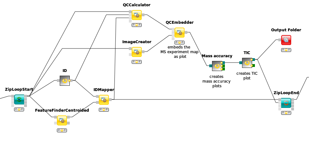
As a start, we will build a basic qcML file for each mzML file in the label-free analysis. We are already creating the two necessary analysis files to build a basic qcML file upon each mzML file, a feature file and an identification file. We use the QCCalculator node from Community > OpenMS > Utilities where also all other QC* nodes will be found. The QCCalculator will create a very basic qcML file in which it will store collected and calculated quality data.
Copy your label-fee quantitation workflow into a new lfq-qc workflow and open it.
Place the QCCalculator node after the
IDMappernode. Being inside the ZipLoop, it will execute for each of the three mzML files the Input node.Connect the first QCCalculator port to the first
ZipLoopStartoutlet port, which will carry the individual mzML files.Connect the last’s ID outlet port (
IDFilteror the ID metanode) to the second QCCalculator port for the identification file.Finally, connect the
IDMapperoutlet to the third QCCalculator port for the feature file.
The created qcML files will not have much to show for, basic as they are. So we will extend them with some basic plots.
First, we will add an 2D overview image of the given mass spectrometry run as you may know it from TOPPView. Add the ImageCreator node from Community Nodes > OpenMS > Utilities. Change the width and heigth parameters to 640x640 as we don’t want it to be too big. Connect it to the first
ZipLoopStartoutlet port, so it will create an image file of the mzML’s contained run.Now we have to embed this file into the qcML file, and attach it to the right QualityParameter. For this, place a QCEmbedder node behind the ImageCreator and connect that to its third inlet port. Connect its first inlet port to the outlet of the QCCalculator node to pass on the qcML file. Now change the parameter cv_acc to QC:0000055 which designates the attached image to be of type QC:0000055 - MS experiment heatmap. Finally, change the parameter qp_att_acc to QC:0000004, to attach the image to the QualityParameter QC:0000004 - MS acquisition result details.
For a reference of which CVs are already defined for qcML, have a look at the following link.
There are two other basic plots which we almost always might want to look at before judging the quality of a mass spectrometry run and its identifications: the total ion current (TIC) and the PSM mass error (Mass accuracy), which we have available as pre-packaged QC metanodes.
Task
Import the workflow from
Copy the Mass accuracy metanode into the workflow behind the QCEmbedder node and connect it. The qcML will be passed on and the Mass accuracy plots added. The information needed was already collected by the QCCalculator.
Do the same with the TIC metanode so that your qcML file will get passed on and enriched on each step.
R Dependencies: This section requires that the R packages ggplot2 and scales are both installed. This is the same procedure as in this section. In case that you use an R installation where one or both of them are not yet installed, open the R Snippet nodes inside the metanodes you just used (double-click). Edit the script in the R Script text editor from:
#install.packages("ggplot2")
#install.packages("scales")
to
install.packages("ggplot2")
install.packages("scales")
Press Eval script to execute the script.
|
|---|
Figure 51: Basic QC setup within a LFQ workflow. |
Note
To have a peek into what our qcML now looks like for one of the ZipLoop iterations, we can add an Output Folder node from Community Nodes > GenericKnimeNodes > IO and set its destination parameter to somewhere we want to find our intermediate qcML files in, for example tmp > qcxlfq. If we now connect the last metanode with the Output Folder and restart the workflow, we can start inspecting the qcML files.
Task
Find your first created qcML file and open it with the browser (not IE), and the contained QC parameters will be rendered for you.
Adding brand new QC metrics
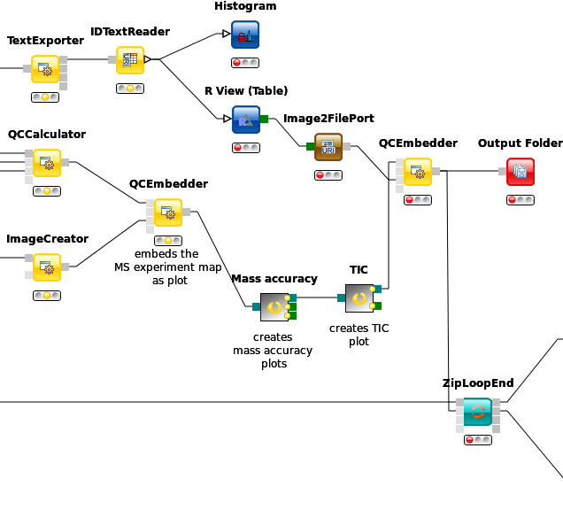
We can also add brand new QC metrics to our qcML files. Remember the Histogram you added inside the ZipLoop during the label-free quantitation section? Let’s imagine for a moment this was a brand new and utterly important metric and plot for the assessment of your analyses quality. There is an easy way to integrate such new metrics into your qcMLs. Though the Histogram node cannot pass its plot to an image, we can do so with a R View (table).
Add an R View (table) next to the IDTextReader node and connect them.
Edit the R View (table) by adding the R Script according to this:
 #install.packages("ggplot2")
library("ggplot2")
ggplot(knime.in, aes(x=peptide_charge)) +

 geom_histogram(binwidth=1, origin =-0.5) +
 scale_x_discrete() +

 ggtitle("Identified peptides charge histogram") +
 ylab("Count")
This will create a plot like the Histogram node on peptide_charge and pass it on as an image.
Now add and connect a Image2FilePort node from Community Nodes > GenericKnimeNodes > Flow to the R View (table).
We can now use a QCEmbetter node like before to add our new metric plot into the qcML.
After looking for an appropriate target from the following link, we found that we can attach our plot to the MS identification result details by setting the parameter
qp_att_acctoQC:0000025, as we are plotting the charge histogram of our identified peptides.To have the plot later displayed properly, we assign it the parameter
cv_accofQC:0000051, a generic plot. Also we made sure in the R Script, that our plot carries a caption so that we know which is which, if we had more than one new plot.Now we redirect the QCEmbedders output to the
Output Folderfrom before and can have a look at how our qcML is coming along after restarting the workflow.
|
|---|
Figure 52: QC with new metric. |
Set QC metrics
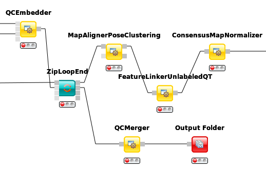
Besides monitoring the quality of each individual mass spectrometry run analysis, another capability of QC with OpenMS and qcML is to monitor the complete set. The easiest control is to compare mass spectrometry runs which should be similar, e.g. technical replicates, to spot any aberrations in the set. For this, we will first collect all created qcML files, merge them together and use the qcML onboard set QC properties to detect any outliers.
Connect the QCEmbedders output from last section to the ZipLoopEnds second input port.
The corresponding output port will collect all qcML files from each ZipLoop iteration and pass them on as a list of files.
Now we add a QCMerger node after the
ZipLoopEndand feed it that list of qcML files. In addition, we set its parametersetnameto give our newly created set a name - sayspikein_replicates.To inspect all the QCs next to each other in that created qcML file, we have to add a new
Output Folderto which we can connect the QCMerger output.
When inspecting the set-qcML file in a browser, we will be presented another overview. After the set content listing, the basic QC parameters (like number of identifications) are each displayed in a graph. Each set member (or run) has its own section on the x-axis and each run is connected with that graph via a link in the mouseover on one of the QC parameter values.
|
|---|
Figure 53: QC set creation from ZipLoop. |
Task
For ideas on new QC metrics and parameters, as you add them in your qcML files as generic parameters, feel free to contact us, so we can include them in the CV.