Feature Detection
For quantitation, the FeatureFinder tools are used. They extract the features from profile data or centroided data. TOPP offers different types of FeatureFinders:
FeatureFinderIsotopeWavelet
Description
The algorithm has been designed to detect features in raw MS data sets. The current implementation is only able to handle MS1 data. An extension handling also tandem MS spectra is under development. The method is based on the isotope wavelet, which has been tailored to the detection of isotopic patterns following the averagine model. For more information about the theory behind this technique, please refer to Hussong et al.: “Efficient Analysis of Mass Spectrometry Data Using the Isotope Wavelet” (2007).
Attention
This algorithm features no “modelling stage”, since the structure of the isotopic pattern is explicitly coded by the wavelet itself. The algorithm also works for 2D maps (in combination with the so-called sweep-line technique (Schulz-Trieglaff et al.: “A Fast and Accurate Algorithm for the Quantification of Peptides from Mass Spectrometry Data” (2007))). The algorithm could originally be executed on (several) high-speed CUDA graphics cards. Tests on real-world data sets revealed potential speedups beyond factors of 200 (using 2 NVIDIA Tesla cards in parallel). Support for CUDA was removed in OpenMS due to maintenance overhead. Please refer to Hussong et al.: “Highly accelerated feature detection in proteomics data sets using modern graphics processing units” (2009) for more details on the implementation.
Seeding
Identification of regions of interest by convolving the signal with the wavelet function. A score, measuring the closeness of the transform to a theoretically determined output function, finally distinguishes potential features from noise.
Extension
The extension is based on the sweep-line paradigm and is done on the fly after the wavelet transform.
Modelling
None (explicitly done by the wavelet).
FeatureFinderCentroided
Description
This is an algorithm for feature detection based on peak data. In contrast to the other algorithms, it is based on peak/stick data, which makes it applicable even if no profile data is available. Another advantage is its speed due to the reduced amount of data after peak picking.
Seeding
It identifies interesting regions by calculating a score for each peak based on
the significance of the intensity in the local environment.
RT dimension: the quality of the mass trace in a local RT window.
m/z dimension: the quality of fit to an averagine isotope model.
Extension
The extension is based on a heuristics – the average slope of the mass trace for RT dimension, the best fit to averagine model in m/z dimension.
Modelling
In model fitting, the retention time profile (Gaussian) of all mass traces is fitted to the data at the same time. After fitting, the data is truncated in RT and m/z dimension. The reported feature intensity is based on the fitted model, rather than on the (noisy) data.
Example
For this example the file LCMS-centroided.mzML from the examples data is used (File > Open example data). In order
to adapt the algorithm to the data, some parameters have to be set.
Intensity
The algorithm estimates the significance of peak intensities in a local environment. Therefore, the HPLC-MS map is
divided into n times n regions. Set the intensity:bins parameter to 10 for the whole map. For a small region, set
it to 1.
Mass trace
For the mass traces, define the number of adjacent spectra in which a mass has to occur (mass_trace:min_spectra). In
order to compensate for peak picking errors, missing peaks can be allowed (mass_trace:max_missing) and a tolerated
mass deviation must be set (mass_trace:mz_tolerance).
Isotope pattern
The expected isotopic intensity pattern is estimated from an averagene amino acid composition. The algorithm searches
all charge states in a defined range (isotopic_pattern:change_min to isotopic_pattern:change_max). Just as for mass
traces, a tolerated mass deviation between isotopic peaks has to be set (isotopic_pattern:mz_tolerance).
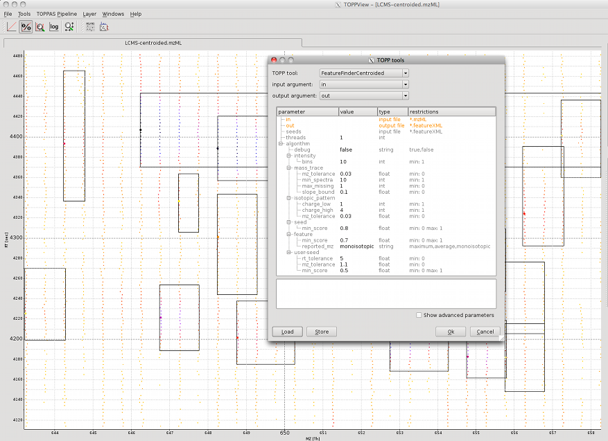
The image shows the centroided peak data and the found peptide features. The used parameters can be found in the TOPP tools dialog.