MSStats

R integration

KNIME provides a large number of nodes for a wide range of statistical analysis, machine learning, data processing, and visualization. Still, more recent statistical analysis methods, specialized visualizations or cutting edge algorithms may not be covered in KNIME. In order to expand its capabilities beyond the readily available nodes, external scripting languages can be integrated. In this tutorial, we primarily use scripts of the powerful statistical computing language R. Note that this part is considered advanced and might be difficult to follow if you are not familiar with R. In this case you might skip this part.

R View (Table) allows to seamlessly include R scripts into KNIME. We will demonstrate on a minimal example how such a script is integrated.

Task

First we need some example data in KNIME, which we will generate using the Data Generator node (IO > Other > Data Generator). You can keep the default settings and execute the node. The table contains four columns, each containing random coordinates and one column containing a cluster number (Cluster_0 to Cluster_3). Now place a R View (Table) node into the workflow and connect the upper output port of the Data Generator node to the input of the R View (Table) node. Right-click and configure the node. If you get an error message like Execute failed: R_HOME does not contain a folder with name ’bin’. or Execution failed: R Home is invalid.: please change the R settings in the preferences. To do so open File > Preferences > KNIME > R and enter the path to your R installation (the folder that contains the bin directory. e.g., C:▸Program Files▸R▸R-3.4.3).

If you get an error message like: ”Execute failed: Could not find Rserve package. Please install it in your R installation by running ”install.packages(’Rserve’)”.” You may need to run your R binary as administrator (In windows explorer: right-click ”Run as administrator”) and enter install.packages(’Rserve’) to install the package.

If R is correctly recognized we can start writing an R script. Consider that we are interested in plotting the first and second coordinates and color them according to their cluster number. In R this can be done in a single line. In the R view (Table) text editor, enter the following code:

plot(x=knime.in$Universe_0_0, y=knime.in$Universe_0_1, main="Plotting column Universe_0_0 vs. Universe_0_1", col=knime.in$"Cluster Membership")

Explanation: The table provided as input to the R View (Table) node is available as R data.frame with name knime.in. Columns (also listed on the left side of the R View window) can be accessed in the usual R way by first specifying the data.frame name and then the column name (e.g., knime.in$Universe_0_0). plot is the plotting function we use to generate the image. We tell it to use the data in column Universe_0_0 of the dataframe object knime.in (denoted as knime.in$Universe_0_0) as x-coordinate and the other column knime.in$Universe_0_1 as y-coordinate in the plot. main is simply the main title of the plot and col the column that is used to determine the color (in this case it is the Cluster Membership column).

Now press the Eval script and Show plot buttons.

Note

Note that we needed to put some extra quotes around Cluster Membership. If we omit those, R would interpret the column name only up to the first space (knime.in$Cluster) which is not present in the table and leads to an error. Quotes are regularly needed if column names contain spaces, tabs or other special characters like $ itself.

Using MSstats in a KNIME workflow

The R package MSstats can be used for statistical relative quantification of proteins and peptides in mass spectrometry-based proteomics. Supported are label-free as well as labeled experiments in combination with data-dependent, targeted and data independent acquisition. Inputs can be identified and quantified entities (peptides or proteins) and the output is a list of differentially abundant entities, or summaries of their relative abundance. It depends on accurate feature detection, identification and quantification which can be performed e.g. by an OpenMS workflow. MSstats can be used for data processing & visualization, as well as statistical modeling & inference. Please see [1] and the MSstats website for further information.

Identification and quantification of the iPRG2015 data with subsequent MSstats analysis

Here, we describe how to use OpenMS and MSstats for the analysis of the ABRF iPRG2015 dataset[2].

Note

Reanalysing the full dataset from scratch would take too long. In the following tutorial, we will focus on just the conversion process and the downstream analysis.

Dataset

The iPRG (Proteome Informatics Research Group) dataset from the study in 2015, as described in [2], aims at evaluating the effect of statistical analysis software on the accuracy of results on a proteomics label-free quantification experiment. The data is based on four artificial samples with known composition (background: 200 ng S. cerevisiae). These were spiked with different quantities of individual digested proteins, whose identifiers were masked for the competition as yeast proteins in the provided database (see Table 1).

Table 1: Samples (background: 200 ng S. cerevisiae) with spiked-in proteins
in different quantities [fmols]

				Samples
	Name	Origin	Molecular Weight	1	2	3	4
A	Ovalbumin	Egg White	45 KD	65	55	15	2
B	Myoglobin	Equine Heart	17 KD	55	15	2	65
C	Phosphorylase b	Rabbit Muscle	97 KD	15	2	65	55
D	Beta-Glactosidase	Escherichia Coli	116 KD	2	65	55	15
E	Bovine Serum Albumin	Bovine Serum	66 KD	11	0.6	10	500
F	Carbonic Anhydrase	Bovine Erythrocytes	29 KD	10	500	11	0.6

Identification and quantification

Figure 18: KNIME data analysis of iPRG LFQ data.

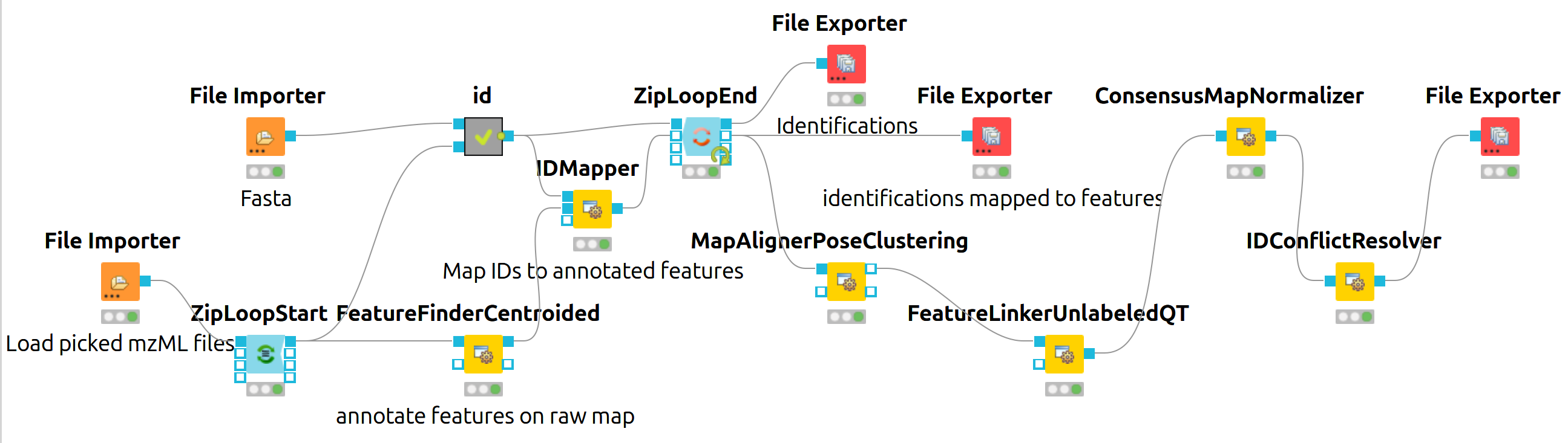
The iPRG LFQ workflow (Fig. 18) consists of an identification and a quantification part. The identification is achieved by searching the computationally calculated MS2 spectra from a sequence database (File Importer node, here with the given database from iPRG: ExampleData▸iPRG2015▸database▸iPRG2015targetdecoynocontaminants.fasta against the MS2 from the original data (Input Files node with all mzMLs following ExampleData▸iPRG2015▸datasets▸JD06232014sample*.mzML using the CometAdapter.

Note

If you want to reproduce the results at home, you have to download the iPRG data in mzML format and perform peak picking on it or convert and pick the raw data with msconvert.

Afterwards, the results are scored using the FalseDiscoveryRate node and filtered to obtain only unique peptides (IDFilter) since MSstats does not support shared peptides, yet. The quantification is achieved by using the FeatureFinderCentroided node, which performs the feature detection on the samples (maps). In the end the quantification results are combined with the filtered identification results (IDMapper). In addition, a linear retention time alignment is performed (MapAlignerPoseClustering), followed by the feature linking process (FeatureLinkerUnlabledQT). The ConsensusMapNormalizers is used to normalize the intensities via robust regression over a set of maps and the IDConflictResolver assures that only one identification (best score) is associated with a feature. The output of this workflow is a consensusXML file, which can now be converted using the MSStatsConverter (see Conversion and downstream analysis section).

Experimental design

As mentioned before, the downstream analysis can be performed using MSstats. In this case, an experimental design has to be specified for the OpenMS workflow. The structure of the experimental design used in OpenMS in case of the iPRG dataset is specified in Table 2.

Table 2: OpenMS Experimental design for the iPRG2015 dataset.

Fraction_Group	Fraction	Spectra_Filepath	Label	Sample
1	1	Sample1-A	1	1
2	1	Sample1-B	1	2
3	1	Sample1-C	1	3
4	1	Sample2-A	1	4
5	1	Sample2-B	1	5
6	1	Sample2-C	1	6
7	1	Sample3-A	1	7
8	1	Sample3-B	1	8
9	1	Sample3-C	1	9
10	1	Sample4-A	1	10
11	1	Sample4-B	1	11
12	1	Sample4-C	1	12
Sample	MSstats_Condition	MSstats_BioReplicate
1	1	1
2	1	2
3	1	3
4	2	4
5	2	5
6	2	6
7	3	7
8	3	8
9	3	9
10	4	10
11	4	11
12	4	12

An explanation of the variables can be found in Table 3.

Table 3: Explanation of the column of the experimental design table

variables	value
Fraction_Group	Index used to group fractions and source files.
Fraction	1st, 2nd, .., fraction. Note: All runs must have the same number of fractions.
Spectra_Filepath	Path to mzML files
Label	label-free: always 1
	TMT6Plex: 1...6
	SILAC with light and heavy: 1..2
Sample	Index of sample measured in the specified label X, in fraction Y of fraction group Z.
Conditions	Further specification of different conditions (e.g. MSstats_Condition; MSstats_BioReplicate)

The conditions are highly dependent on the type of experiment and on which kind of analysis you want to perform. For the MSstats analysis the information which sample belongs to which condition and if there are biological replicates are mandatory. This can be specified in further condition columns as explained in Table 3. For a detailed description of the MSstats-specific terminology, see their documentation e.g. in the R vignette.

Conversion and downstream analysis

Conversion of the OpenMS-internal consensusXML format (which is an aggregation of quantified and possibly identified features across several MS-maps) to a table (in MSstats-conformant CSV format) is very easy. First, create a new KNIME workflow. Then, run the MSStatsConverter node with a consensusXML and the manually created (e.g. in Excel) experimental design as inputs (loaded via File Importer nodes). The first input can be found in:

ExampleData▸iPRG2015▸openmsLFQResults▸iPRGlfq.consensusXML

This file was generated by using the Workflows▸openmsLFQiPRG2015.knwf workflow (seen in Fig. 18). The second input is specified in:

ExampleData▸iPRG2015▸experimentaldesign.tsv

Adjust the parameters in the config dialog of the converter to match the given experimental design file and to use a simple summing for peptides that elute in multiple features (with the same charge state, i.e. m/z value).

parameter	value
msstats_bioreplicate	MSstats_Bioreplicate
msstats_condition	MSstats_Condition
labeled_reference_peptides	false
retention_time_summarization_method (advanced)	sum

The downstream analysis of the peptide ions with MSstats is performed in several steps. These steps are reflected by several KNIME R nodes, which consume the output of MSStatsConverter. The outline of the workflow is shown in Figure 19.

Figure 19: MSstats analysis using KNIME. The individual steps (Preprocessing, Group Comparisons, Result Data Renaming, and Export) are split among several consecutive nodes.

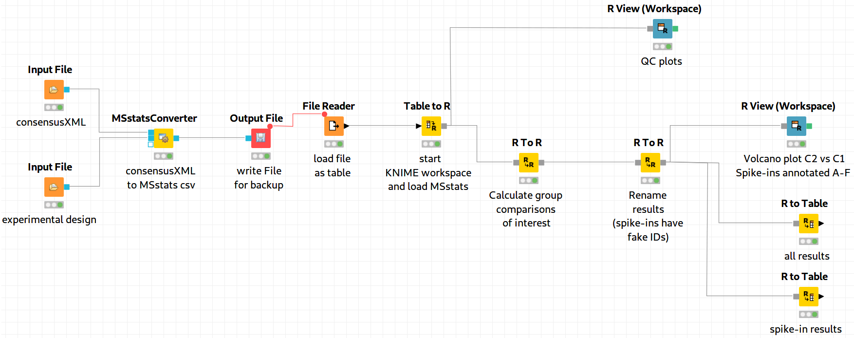
We load the file resulting from MSStatsConverter either by saving it with an Output File node and reloading it with the File Reader. Alternatively, for advanced users, you can use a URI Port to Variable node and use the variable in the File Reader config dialog (V button - located on the right of the Browse button) to read from the temporary file.

Preprocessing

The first node (Table to R) loads MSstats as well as the data from the previous KNIME node and performs a preprocessing step on the input data. The following inline R script ( needs to be pasted into the config dialog of the node):

library(MSstats)
data <- knime.in
quant <- OpenMStoMSstatsFormat(data, removeProtein_with1Feature = FALSE)

The inline R script allows further preparation of the data produced by MSStatsConverter before the actual analysis is performed. In this example, the lines with proteins, which were identified with only one feature, were retained. Alternatively they could be removed. In the same node, most importantly, the following line transforms the data into a format that is understood by MSstats:

processed.quant <- dataProcess(quant, censoredInt = 'NA')

Here, dataProcess is one of the most important functions that the R package provides. The function performs the following steps:

1. Logarithm transformation of the intensities

2. Normalization

3. Feature selection

4. Missing value imputation

5. Run-level summarization

In this example, we just state that missing intensity values are represented by the NA string.

Group Comparison

The goal of the analysis is the determination of differentially-expressed proteins among the different conditions C1-C4. We can specify the comparisons that we want to make in a comparison matrix. For this, let’s consider the following example:

This matrix has the following properties:

• The number of rows equals the number of comparisons that we want to perform, the number of columns equals the number of conditions (here, column 1 refers to C1, column 2 to C2 and so forth).

• The entries of each row consist of exactly one 1 and one -1, the others must be 0.

• The condition with the entry 1 constitutes the enumerator of the log2 fold-change. The one with entry -1 denotes the denominator. Hence, the first row states that we want calculate:

\[ \begin{equation} \log_2 \frac{C_{2}}{C_{1}} \end{equation}\]

We can generate such a matrix in R using the following code snippet in (for example) a new R to R node that takes over the R workspace from the previous node with all its variables:

comparison1<-matrix(c(-1,1,0,0),nrow=1)   
comparison2<-matrix(c(-1,0,1,0),nrow=1)

comparison3<-matrix(c(-1,0,0,1),nrow=1)  
comparison4<-matrix(c(0,-1,1,0),nrow=1)

comparison5<-matrix(c(0,-1,0,1),nrow=1)  
comparison6<-matrix(c(0,0,-1,1),nrow=1)

comparison <- rbind(comparison1, comparison2, comparison3, comparison4, comparison5, comparison6)
row.names(comparison)<-c("C2-C1","C3-C1","C4-C1","C3-C2","C4-C2","C4-C3")

Here, we assemble each row in turn, concatenate them at the end, and provide row names for labeling the rows with the respective condition. In MSstats, the group comparison is then performed with the following line:

test.MSstats <- groupComparison(contrast.matrix=comparison, data=processed.quant)

No more parameters need to be set for performing the comparison.

Result processing

In a next R to R node, the results are being processed. The following code snippet will rename the spiked-in proteins to A,B,C,D,E, and F and remove the names of other proteins, which will be beneficial for the subsequent visualization, as for example performed in Figure 20:

  test.MSstats.cr <- test.MSstats$ComparisonResult   


  # Rename spiked ins to A,B,C....  
  pnames <- c("A", "B", "C", "D", "E", "F")

  names(pnames) <- c(  
  "sp|P44015|VAC2_YEAST",  
  "sp|P55752|ISCB_YEAST",

  "sp|P44374|SFG2_YEAST",  
  "sp|P44983|UTR6_YEAST",  
  "sp|P44683|PGA4_YEAST",

  "sp|P55249|ZRT4_YEAST"  
  )  

  test.MSstats.cr.spikedins <- bind_rows(

  test.MSstats.cr[grep("P44015", test.MSstats.cr$Protein),],

  test.MSstats.cr[grep("P55752", test.MSstats.cr$Protein),],

  test.MSstats.cr[grep("P44374", test.MSstats.cr$Protein),],

  test.MSstats.cr[grep("P44683", test.MSstats.cr$Protein),],

  test.MSstats.cr[grep("P44983", test.MSstats.cr$Protein),],

  test.MSstats.cr[grep("P55249", test.MSstats.cr$Protein),]  
  )  
  # Rename Proteins

  test.MSstats.cr.spikedins$Protein <- sapply(test.MSstats.cr.spikedins$Protein, function(x) {pnames[as.character(x)]})



  test.MSstats.cr$Protein <- sapply(test.MSstats.cr$Protein, function(x) {


    x <- as.character(x)  

    if (x %in% names(pnames)) {


      return(pnames[as.character(x)])  
      } else {  
      return("")

    }
  })

Export

The last four nodes, each connected and making use of the same workspace from the last node, will export the results to a textual representation and volcano plots for further inspection. Firstly, quality control can be performed with the following snippet:

qcplot <- dataProcessPlots(processed.quant, type="QCplot",   
        ylimDown=0,

which.Protein = 'allonly',
width=7, height=7, address=F)

The code for this snippet is embedded in the first output node of the workflow. The resulting boxplots show the log2 intensity distribution across the MS runs. The second node is an R View (Workspace) node that returns a Volcano plot which displays differentially expressed proteins between conditions C2 vs. C1. The plot is described in more detail in the following Result section. This is how you generate it:

groupComparisonPlots(data=test.MSstats.cr, type="VolcanoPlot",

                    width=12, height=12,dot.size = 2,ylimUp = 7,

                    which.Comparison = "C2-C1",
                    address=F)

The last two nodes export the MSstats results as a KNIME table for potential further analysis or for writing it to a (e.g. csv) file. Note that you could also write output inside the Rscript if you are familiar with it. Use the following for an R to Table node exporting all results:

knime.out <- test.MSstats.cr

And this for an R to Table node exporting only results for the spike-ins:

knime.out <- test.MSstats.cr.spikedins

Result

An excerpt of the main result of the group comparison can be seen in Figure 20.

Figure 20: Volcano plots produced by the Group Comparison in MSstats The dotted line indicates an adjusted p-value threshold

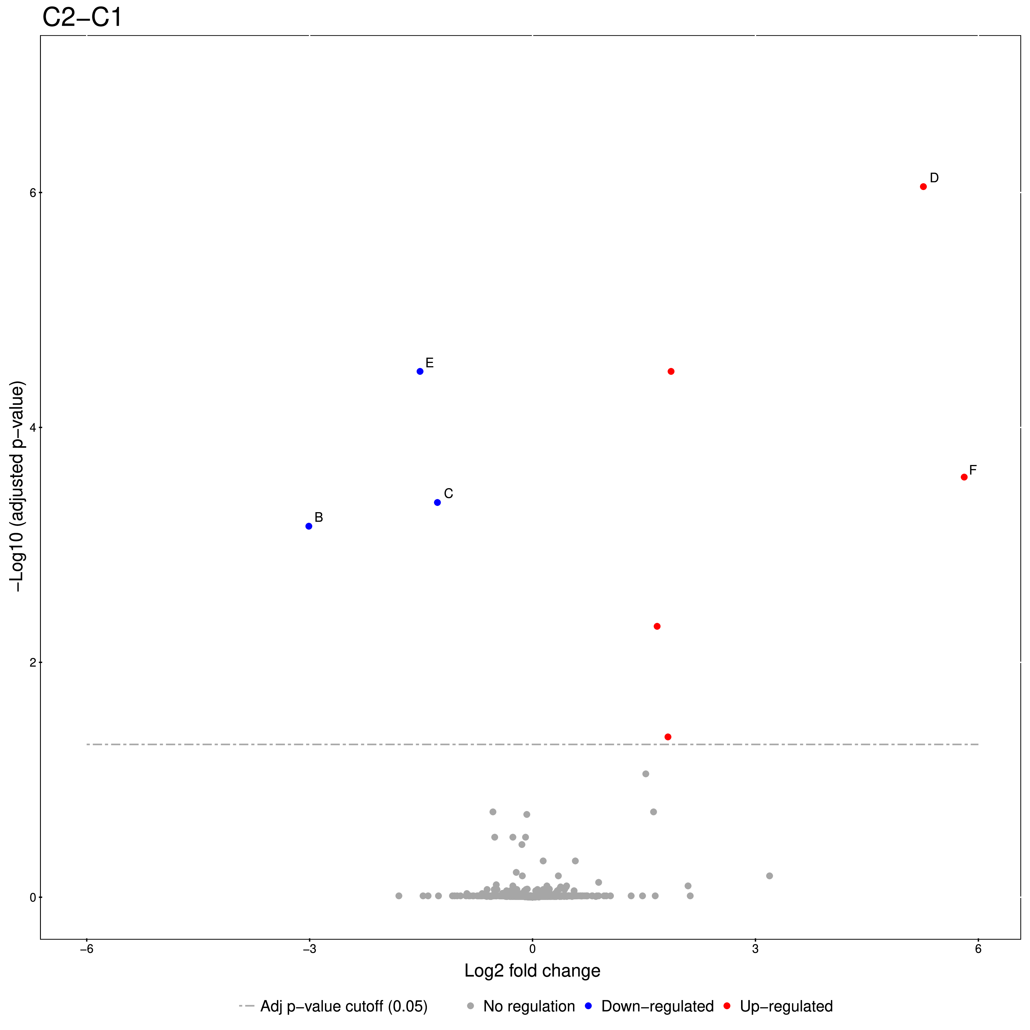
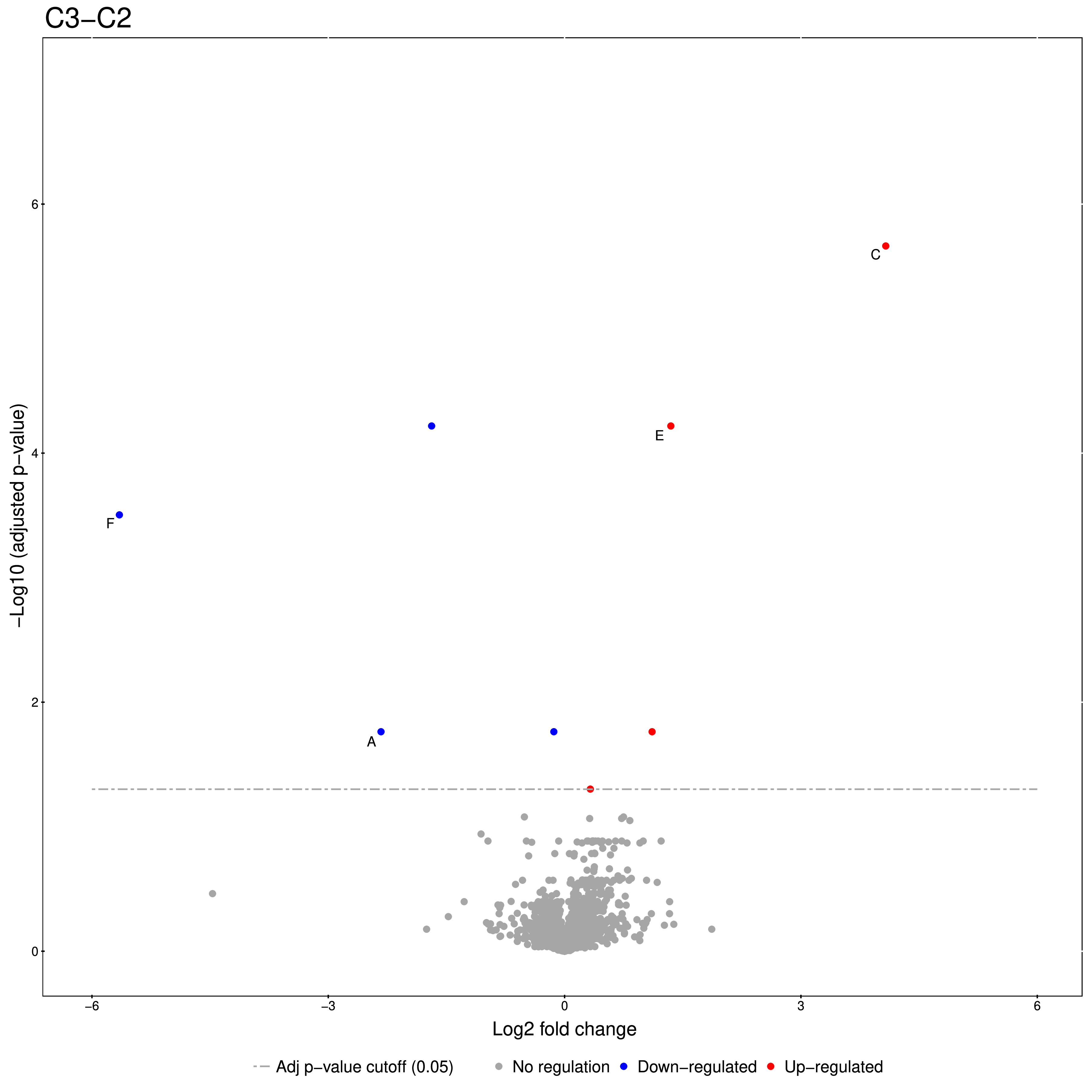
The Volcano plots show differently expressed spiked-in proteins. In the left plot, which shows the fold-change C2-C1, we can see the proteins D and F (sp|P44983|UTR6_YEAST and sp|P55249|ZRT4_YEAST) are significantly over-expressed in C2, while the proteins B,C, and E (sp|P55752|ISCB_YEAST, sp|P55752|ISCB_YEAST, and sp|P44683|PGA4_YEAST) are under-expressed. In the right plot, which shows the fold-change ratio of C3 vs. C2, we can see the proteins E and C (sp|P44683|PGA4_YEAST and sp|P44374|SFG2_YEAST) over-expressed and the proteins A and F (sp|P44015|VAC2_YEAST and sp|P55249|ZRT4_YEAST) under-expressed. The plots also show further differentially-expressed proteins, which do not belong to the spiked-in proteins.

The full analysis workflow can be found under: Workflows▸MSstatsstatPostProcessingiPRG2015.knwf

Isobaric analysis workflow

In the last chapters, we identified and quantified peptides in a label-free experiment.

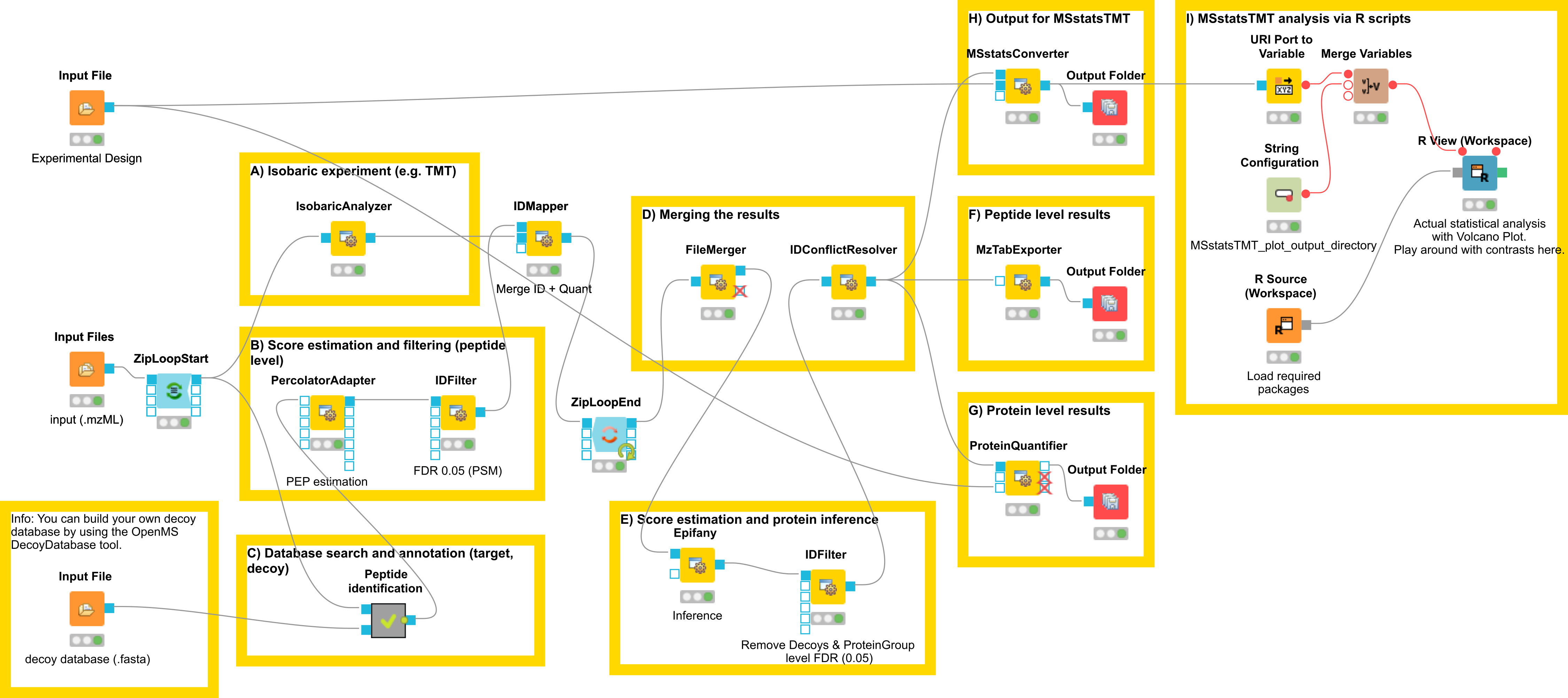
In this section, we would like to introduce a possible workflow for the analysis of isobaric data. Let’s have a look at the workflow (see Fig 23).

Figure 23: Workflow for the analysis of isobaric data

The full analysis workflow can be found here: Workflows▸IdentificationquantificationisobaricinferenceepifanyMSstatsTMT

The workflow has four input nodes. The first for the experimental design to allow for MSstatsTMT compatible export (MSStatsConverter). The second for the .mzML files with the centroided spectra from the isobaric labeling experiment and the third one for the .fasta database used for identification. The last one allows to specify an output path for the plots generated by the R View, which runs MSstatsTMT (I). The quantification (A) is performed using the IsobaricAnalzyer. The tool is able to extract and normalize quantitative information from TMT and iTRAQ data. The values can be assessed from centroided MS2 or MS3 spectra (if available). Isotope correction is performed based on the specified correction matrix (as provided by the manufacturer). The identification © is applied as known from the previous chapters by using database search and a target-decoy database.

To reduce the complexity of the data for later inference the q-value estimation and FDR filtering is performed on PSM level for each file individually (B). Afterwards the identification (PSM) and quantiative information is combined using the IDMapper. After the processing of all available files, the intermediate results are aggregated (FileMerger - D). All PSM results are used for score estimation and protein inference (Epifany) (E). For detailed information about protein inference please see Chaper 4. Then, decoys are removed and the inference results are filtered via a protein group FDR. Peptide level results can be exported via MzTabExporter (F), protein level results can be obtained via the ProteinQuantifier (G) or the results can exported (MSStatsConverter - H) and further processed with the following R pipeline to allow for downstream processing using MSstatsTMT.

Please import the workflow from Workflows▸IdentificationquantificationisobaricinferenceepifanyMSstatsTMT into KNIME via the menu entry File > Import KNIME workflow > Select file and double-click the imported workflow in order to open it. Before you can execute the workflow, you have to correct the locations of the files in the Input Files nodes (don’t forget the one for the FASTA database inside the “ID” meta node). Try and run your workflow by executing all nodes at once.

Excursion MSstatsTMT

The R package MSstatsTMT can be used for protein significance analysis in shotgun mass spectrometry-based proteomic experiments with tandem mass tag (TMT) labeling. MSstatsTMT provides functionality for two types of analysis & their visualization: Protein summarization based on peptide quantification and Model-based group comparison to detect significant changes in abundance. It depends on accurate feature detection, identification and quantification which can be performed e.g. by an OpenMS workflow.

In general, MSstatsTMT can be used for data processing & visualization, as well as statistical modeling. Please see [3] and the MSstats website for further information.

There is also an online lecture and tutorial for MSstatsTMT from the May Institute Workshop 2020.

Dataset and experimental design

We are using the MSV000084264 ground truth dataset, which consists of TMT10plex controlled mixes of different concentrated UPS1 peptides spiked into SILAC HeLa peptides measured in a dilution series https://www.omicsdi.org/dataset/massive/MSV000084264. Figure 24 shows the experimental design. In this experiment, 5 different TMT10plex mixtures – different labeling strategies – were analysed. These were measured in triplicates represented by the 15 MS runs (3 runs each). The example data, database and experimental design to run the workflow can be found here.

Figure 24: Experimental Design

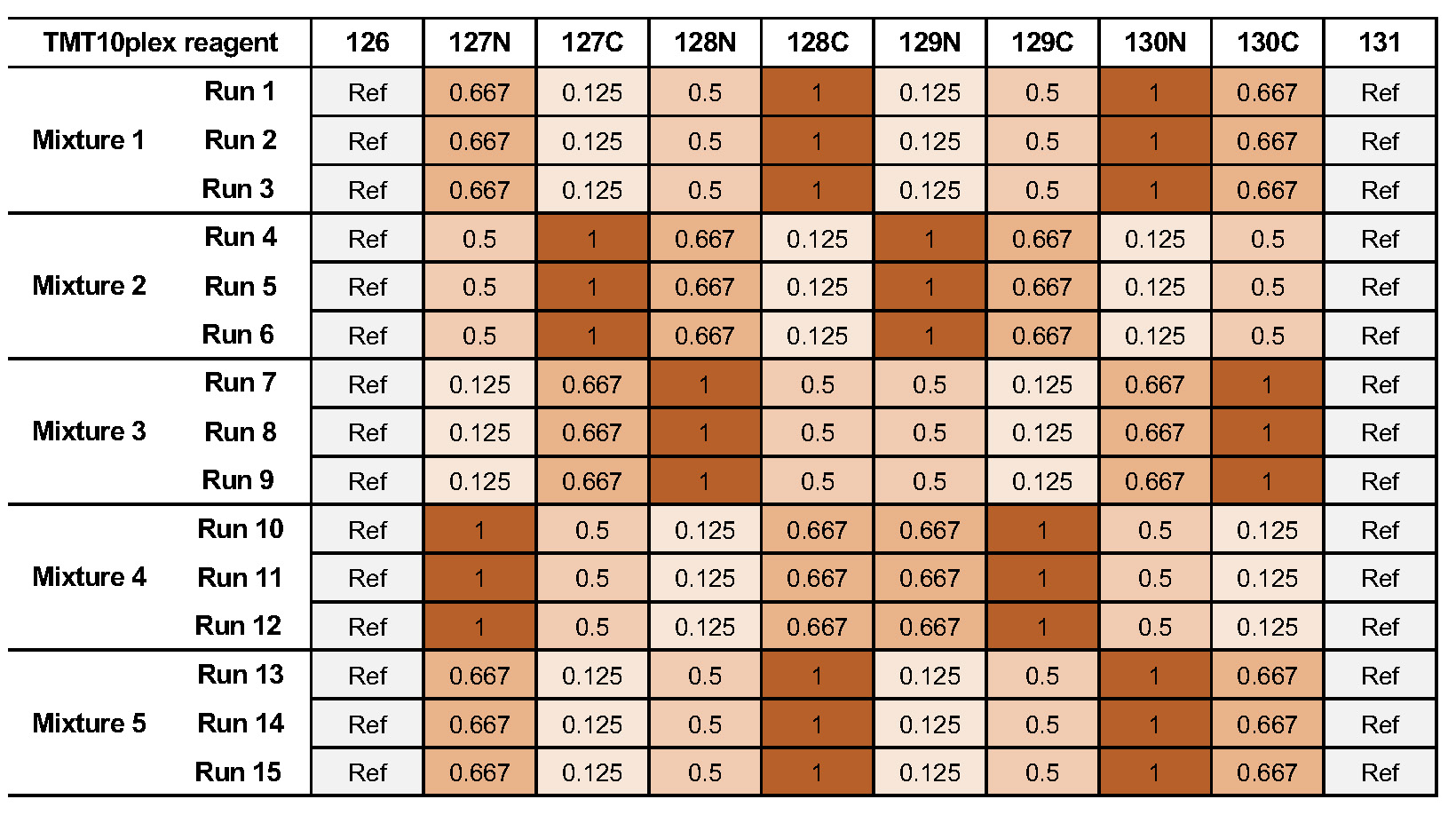
The experimental design in table format allows for MSstatsTMT compatible export. The design is represented by two tables. The first one 4 represents the overall structure of the experiment in terms of samples, fractions, labels and fraction groups. The second one 5 adds to the first by specifying specific conditions, biological replicates as well as mixtures and label for each channel. For additional information about the experimental design please see Table 3.

Table 4: Experimental Design 1

Spectra_Filepath	Fraction	Label	Fraction_Group	Sample
161117_SILAC_HeLa_UPS1_TMT10_SPS_MS3_Mixture1_01.mzML	1	1	1	1
161117_SILAC_HeLa_UPS1_TMT10_SPS_MS3_Mixture1_01.mzML	1	2	1	2
161117_SILAC_HeLa_UPS1_TMT10_SPS_MS3_Mixture1_01.mzML	1	3	1	3
161117_SILAC_HeLa_UPS1_TMT10_SPS_MS3_Mixture1_01.mzML	1	4	1	4
161117_SILAC_HeLa_UPS1_TMT10_SPS_MS3_Mixture1_01.mzML	1	5	1	5
161117_SILAC_HeLa_UPS1_TMT10_SPS_MS3_Mixture1_01.mzML	1	6	1	6
161117_SILAC_HeLa_UPS1_TMT10_SPS_MS3_Mixture1_01.mzML	1	7	1	7
161117_SILAC_HeLa_UPS1_TMT10_SPS_MS3_Mixture1_01.mzML	1	8	1	8
161117_SILAC_HeLa_UPS1_TMT10_SPS_MS3_Mixture1_01.mzML	1	9	1	9
161117_SILAC_HeLa_UPS1_TMT10_SPS_MS3_Mixture1_01.mzML	1	10	1	10
161117_SILAC_HeLa_UPS1_TMT10_SPS_MS3_Mixture1_02.mzML	1	1	2	11
161117_SILAC_HeLa_UPS1_TMT10_SPS_MS3_Mixture1_02.mzML	1	2	2	12
161117_SILAC_HeLa_UPS1_TMT10_SPS_MS3_Mixture1_02.mzML	1	3	2	13
161117_SILAC_HeLa_UPS1_TMT10_SPS_MS3_Mixture1_02.mzML	1	4	2	14
161117_SILAC_HeLa_UPS1_TMT10_SPS_MS3_Mixture1_02.mzML	1	5	2	15
161117_SILAC_HeLa_UPS1_TMT10_SPS_MS3_Mixture1_02.mzML	1	6	2	16
161117_SILAC_HeLa_UPS1_TMT10_SPS_MS3_Mixture1_02.mzML	1	7	2	17
161117_SILAC_HeLa_UPS1_TMT10_SPS_MS3_Mixture1_02.mzML	1	8	2	18
161117_SILAC_HeLa_UPS1_TMT10_SPS_MS3_Mixture1_02.mzML	1	9	2	19
161117_SILAC_HeLa_UPS1_TMT10_SPS_MS3_Mixture1_02.mzML	1	10	2	20
161117_SILAC_HeLa_UPS1_TMT10_SPS_MS3_Mixture1_03.mzML	1	1	3	21
161117_SILAC_HeLa_UPS1_TMT10_SPS_MS3_Mixture1_03.mzML	1	2	3	22
161117_SILAC_HeLa_UPS1_TMT10_SPS_MS3_Mixture1_03.mzML	1	3	3	23
161117_SILAC_HeLa_UPS1_TMT10_SPS_MS3_Mixture1_03.mzML	1	4	3	24
161117_SILAC_HeLa_UPS1_TMT10_SPS_MS3_Mixture1_03.mzML	1	5	3	25
161117_SILAC_HeLa_UPS1_TMT10_SPS_MS3_Mixture1_03.mzML	1	6	3	26
161117_SILAC_HeLa_UPS1_TMT10_SPS_MS3_Mixture1_03.mzML	1	7	3	27
161117_SILAC_HeLa_UPS1_TMT10_SPS_MS3_Mixture1_03.mzML	1	8	3	28
161117_SILAC_HeLa_UPS1_TMT10_SPS_MS3_Mixture1_03.mzML	1	9	3	29
161117_SILAC_HeLa_UPS1_TMT10_SPS_MS3_Mixture1_03.mzML	1	10	3	30

Table 5: Experimental Design 2

Sample	MSstats_Condition	MSstats_BioReplicate	MSstats_Mixture	LabelName
1	Norm	Norm	1	126
2	0.667	0.667	1	127N
3	0.125	0.125	1	127C
4	0.5	0.5	1	128N
5	1	1	1	128C
6	0.125	0.125	1	129N
7	0.5	0.5	1	129C
8	1	1	1	130N
9	0.667	0.667	1	130C
10	Norm	Norm	1	131
11	Norm	Norm	1	126
12	0.667	0.667	1	127N
13	0.125	0.125	1	127C
14	0.5	0.5	1	128N
15	1	1	1	128C
16	0.125	0.125	1	129N
17	0.5	0.5	1	129C
18	1	1	1	130N
19	0.667	0.667	1	130C
20	Norm	Norm	1	131
21	Norm	Norm	1	126
22	0.667	0.667	1	127N
23	0.125	0.125	1	127C
24	0.5	0.5	1	128N
25	1	1	1	128C
26	0.125	0.125	1	129N
27	0.5	0.5	1	129C
28	1	1	1	130N
29	0.667	0.667	1	130C
30	Norm	Norm	1	131

After running the worklfow, the MSStatsConverter will convert the OpenMS output in addition with the experimental design to a file (.csv) which can be processed by using MSstatsTMT.

MSstatsTMT analysis

Here, we depict the analysis by MSstatsTMT using a segment of the isobaric analysis workflow (Fig. 25). The segment is available as Workflows▸MSstatsTMT.knwf.

Figure 25: MSstatsTMT workflow segment

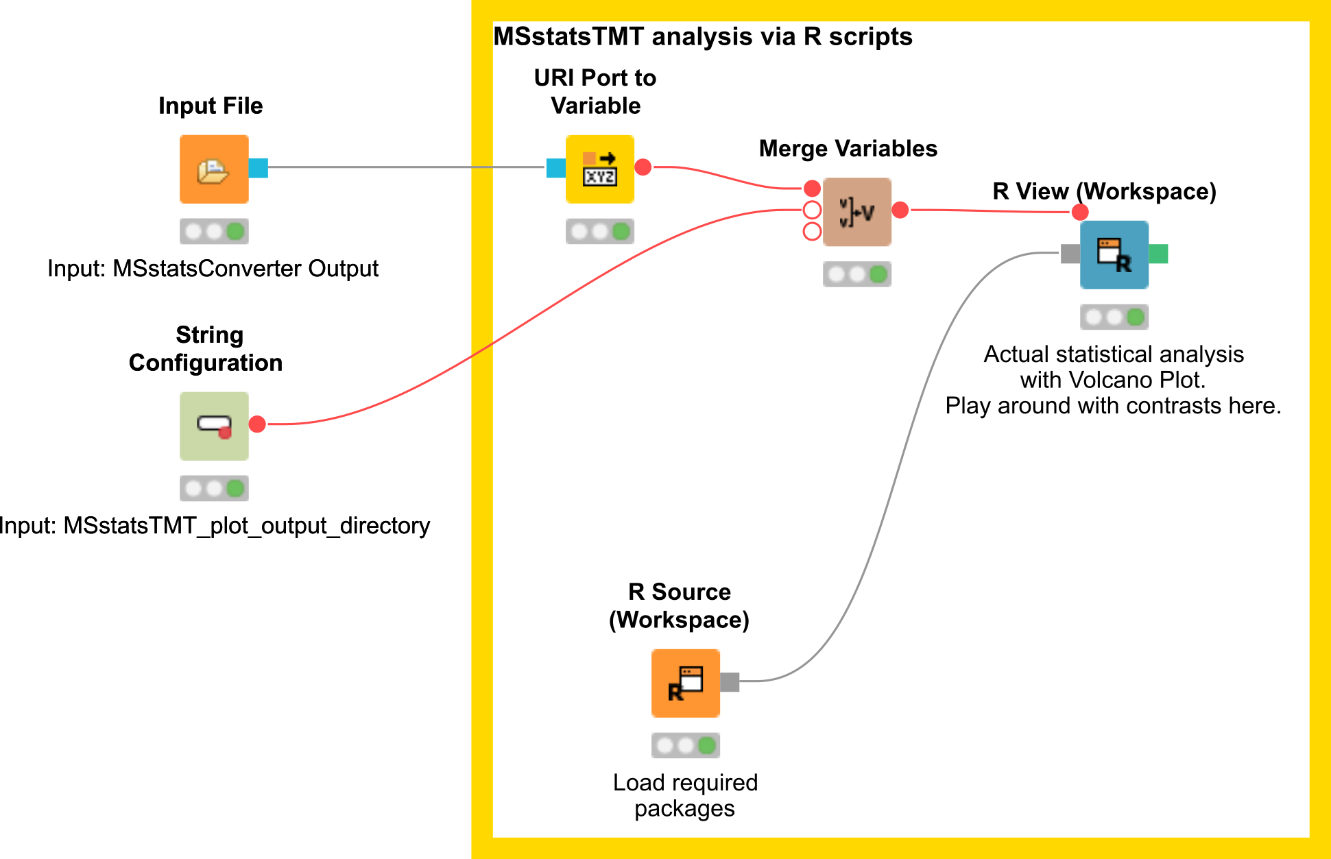
There are two input nodes, the first one takes the result (.csv) from the MSStatsConverter and the second a path to the directory where the plots generated by MSstatsTMT should be saved. The R source node loads the required packages, such as dplyr for data wrangling, MSstatsTMT for analysis and MSstats for plotting. The inputs are further processed in the R View node.

Here, the data of the File Importer is loaded into R using the flow variable [”URI-0”]:

file <- substr(knime.flow.in[["URI-0"]], 6, nchar(knime.flow.in[["URI-0"]]))

MSstatsConverter_OpenMS_out <- read.csv(file)
data <- MSstatsConverter_OpenMS_out

The OpenMStoMSstatsTMTFormat function preprocesses the OpenMS report and converts it into the required input format for MSstatsTMT, by filtering based on unique peptides and measurements in each MS run.

processed.data <- OpenMStoMSstatsTMTFormat(data)

Afterwards different normalization steps are performed (global, protein, runs) as well as data imputation by using the msstats method. In addition peptide level data is summarized to protein level data.

quant.data <- proteinSummarization(processed.data,   
                                  method="msstats",

                                  global_norm=TRUE,  
                                  reference_norm=TRUE,

                                  MBimpute = TRUE,  
                                  maxQuantileforCensored = NULL,

                                  remove_norm_channel = TRUE,
                                  remove_empty_channel =  TRUE)

There a lot of different possibilities to configure this method please have a look at the MSstatsTMT package for additional detailed information.

The next step is the comparions of the different conditions, here either a pairwise comparision can be performed or a confusion matrix can be created. The goal is to detect and compare the UPS peptides spiked in at different concentrations.

# prepare contrast matrix   
unique(quant.data$Condition)  

comparison<-matrix(c(-1,0,0,1,

                     0,-1,0,1,  
                     0,0,-1,1,

                     0,1,-1,0,  
                     1,-1,0,0), nrow=5, byrow = T)  


# Set the names of each row  
row.names(comparison)<- contrasts <- c("1-0125",

                                       "1-05",  
                                       "1-0667",

                                       "05-0667",  
                                       "0125-05")

# Set the column names
colnames(comparison)<- c("0.125", "0.5", "0.667", "1")

The constructed confusion matrix is used in the groupComparisonTMT function to test for significant changes in protein abundance across conditions based on a family of linear mixed-effects models in TMT experiments.

data.res <- groupComparisonTMT(data = quant.data,   
                               contrast.matrix = comparison,

                               moderated = TRUE, # do moderated t test

                               adj.method = "BH") # multiple comparison adjustment
data.res <- data.res %>% filter(!is.na(Protein))

In the next step the comparison can be plotted using the groupComparisonPlots function by MSstats.

library(MSstats)  
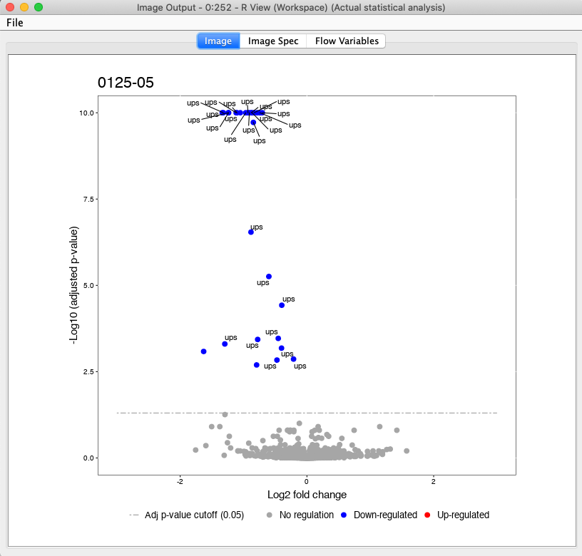
groupComparisonPlots(data=data.res.mod, type="VolcanoPlot", address=F, which.Comparison = "0125-05", sig = 0.05)

Here, we have a example output of the R View, which depicts the significant regulated UPS proteins in the comparison of 125 to 05 (Fig. 26).

Figure 26: Volcanoplot of the group comparison regarding 0125 to 05

All plots are saved to the in the beginning specified output directory in addition.

Note

The isobaric analysis does not always has to be performed on protein level, for example for phosphoproteomics studies one is usually interested on the peptide level - in addition inference on peptides with post-translational modification is not straight forward. Here, we present and additonal workflow on peptide level, which can potentially be adapted and used for such cases. Please see Workflows▸IdentificationquantificationisobaricMSstatsTMT

References

[1]

A. Chawade, M. Sandin, J. Teleman, J. Malmström, and F. Levander, Data Processing Has Major Impact on the Outcome of Quantitative Label-Free LC-MS Analysis, Journal of Proteome Research 14(2), 676–687 (2015), PMID: 25407311, arXiv:http://dx.doi.org/10.1021/pr500665j, doi:10.1021/pr500665j. 30

[2] (1,2)

M. Choi, Z. F. Eren-Dogu, C. Colangelo, J. Cottrell, M. R. Hoopmann, E. A. Kapp, S. Kim, H. Lam, T. A. Neubert, M. Palmblad, B. S. Phinney, S. T. Weintraub, B. MacLean, and O. Vitek, ABRF Proteome Informatics Research Group (iPRG) 2015 Study: Detection of Differentially Abundant Proteins in Label-Free Quantitative LC-MS/MS Experiments, J. Proteome Res. 16(2), 945–957 (2017), doi: 10.1021/acs.jproteome.6b00881. 40

[3]

T. Huang, M. Choi, S. Hao, and O. Vitek, MSstatsTMT: Protein Significance Analysis in shotgun mass spectrometry-based proteomic experiments with tandem mass tag (TMT) labeling., (2020), doi:10.18129/B9.bioc.MSstatsTMT. 55